Team:British Columbia/modeling description

Introduction

We developed a mathematical model that describes the dynamics of the biofilm structure (in terms of bacterial population size) and the interactions among the major components, including the engineered phage and DispersinB (DspB) protein. We used numerical simulations to predict the impact of phage and DspB release on the biofilm. We also investigated the weight of each parameter to the design of our system using sensitivity analysis. Using our model, we explored scenarios of biofilm degradation that may be encountered in the real world. We implemented our model in a Java program called PhilmIt-v1.

Basic Biofilm Geometry

The biofilm system assumes a simple planar geometry characterized by depth, D, and cross-sectional area, A (Figure 1). The density and distribution of the biofilm bacterial population, extracellular polymeric substance (EPS), and dissolved components (e.g. AIP and metabolites) are uniform throughout the biofilm structure. Assuming that each biofilm bacterium occupies a spherical volume of diameter, d, and the surrounding EPS extends this volume by a constant, α, each bacterium takes up a cubic volume of (α + d)³. The total bacterial population in a biofilm can be estimated:

The carrying capacity determines the maximum biofilm thickness, and therefore can be coarsely estimated by letting D equal to the maximum thickness in Equation 1.

Biofilm Bacteria

The total bacterial population, B_T, is divided into two subpopulations: 1) the carrier bacteria, B_i, which are infected with the engineered phage and 2) the non-carrier bacteria, B_u, which are uninfected but susceptible to phage infection upon exposure. The total population, B_T, undergo logistic growth at rate ρ_T limited by the carrying capacity, K; the uninfected, B_u, and infected, B_i, subpopulations grow at rates ρ_u and ρ_i, respectively (the equations describing these components will be discussed in the next section). We separate the carrier bacteria subpopulation further into two subpopulations: 1) the bacteria infected with the phage in latent phase, B_l, and 2) those infected with the phage in lytic phase, B_L. The flow diagram in Figure 2 summarizes the hierarchical relationships among components of the biofilm population.

Phage Particles

Initially, only the engineered S. aureus bacteria will be introduced to the biofilm. In response to the presence of AIP, they will generate and release the first batch of phage particles. A proportion of these phage particles, κ, will successfully infect and integrate its genetic information into the host genome. Once infected, a bacterium is subject to lysis probability of λ; upon lysis, the bacterium will release R number of phage particles. The dynamics of the phage particles is also governed by half-life, t_1/2, and follows this differential equation, where δ is the portion of phage remaining in the biofilm structure after diffusion (described in detail below):

Phage Diffusion and Invasion

Lysis of the infected host cells forms a pool of newly produced phage particles. This phage population diffuses out 1) towards the bulk liquid at rate r_out or 2) into the biofilm structure through EPS at rate r_in. We assume that the new phage pool is concentrated in a defined layer immediately after lysis. This layer serves as the initial point of diffusion. The diffusion of phage particles into the biofilm can be modeled by Fick’s second law of diffusion, where φ is the phage concentration and x the distance from the boundary of the phage-infested layer (here, it is interpreted as the thickness of the new phage-infested layer):

Equations
Let us redefine the concentration, φ, to be relative to the initial phage concentration, φ₀, at time t = 0 such that φ_r = φ / φ₀:

Equations
Solving for φ_r, we derive:

The distance of phage diffusion within one time step (i.e. from t = 0 to t = 1) can be estimated by letting φ_r = 0 and solving for x, which is dependent on the constant, θ, and diffusion coefficient, r_in (Equation 10.1) Note that the integral cannot be solved analytically in closed form. Numerical methods such as the adaptive Simpson quadrature are required to estimate it.

Equations
Since we are treating this as a one-dimensional problem, the distance of phage diffusion can be roughly estimated by the diffusion length for a time period, dt:

For simplicity, we will implement this equation in our simulations.

Equations
This distance reflects the depth of the phage-infested layer and is related to the proportion of the total biofilm susceptible to infection. We simplify this relationship by using information about the geometry of the biofilm bacteria and biofilm structure. The following represents the relationship between the depth of the remaining biofilm (i.e. not disintegrated by phage) and the total biofilm population.

Dispersal Process

The phage population introduced to the boundary layer will infect the biofilm starting at the exposed biofilm surface. A portion of the total biofilm population, ε, is susceptible to infection due to limited phage access to the biofilm. Because we assume that the composition of biofilm is homogeneous, the portion of susceptible biofilm is related to the depth of phage invasion, z, and the depth of the phage-infested layer, x:

Equation
Moreover, a portion of the non-carrier population, ε_u of B_u, can be infected:

Equation
The uninfected bacteria and the infected undergo growth at rates, ρ_u and ρ_i, respectively. The growth of both subpopulations will contribute to attaining the maximum thickness of the total biofilm. Thus, the dynamics of the two biofilm subpopulations can be described by the following differential equations:

Equations
The sum of the rate terms of the subpopulations yields the differential equation describing the dynamics of the total bacterial population. Note that the logistic growth component is proportionally separated for the subpopulations (Equations x and x). Here, the term for overall biofilm population decline is primarily dependent on B_i.

The following differential equations describe the dynamics of the two infected subpopulations, where p is the portion of latent bacteria, π the rate of transition from latent to lytic phase, and λ the rate of host lysis:

DspB Activity

The production of DspB enzymes is coupled with phage production since they are both activated via the same signal pathway. The concentration of DspB enzymes in the EPS is subject to diffusion forces similar to those acting on the phage particles. The dynamics of extracellular DspB concentration is therefore, where S is the amount of DspB released per host lysis:

Equation
The lysis release of DspB enzymes promotes phage invasion by facilitating access into the biofilm structure due to their EPS-degrading activity. Therefore, DspB increases the diffusion rate of the phage particles into biofilm. The diffusion rate is related to the concentration of DspB in the phage-infested layer, where Y is the proportionality constant:

AIP Activity

Biofilms maintain their extracellular concentration of AIP at [AIP]_max. Here, we assume that AIP is being secreted by the biofilm bacteria at rate which is a function of the total biofilm population and degrades at rate γ. The dynamics of AIP concentration is assumed to behave more or less logistically:

Equation
The activation of phage production and dspB transcription is dependent on the extracellular concentration of AIP. We engineered the system so that it responds to a certain threshold level of AIP, [AIP]_thres, below which phage production and dspB transcription ceases (i.e. R = 0 and S = 0). Modifying Equation, we derive conditional differential equations describing phage dynamics:

Equation
Furthermore, AIP-dependent dynamics of DspB production entails, where when extracellular AIP concentration falls below the activation threshold. Since dspB transcription is coupled with phage generation, we derive differential equations of DspB dynamics similar to those of phage dynamics:

Output

The progress and outcome of phage invasion can be monitored by the populations of the biofilm and the phage. Hence, the output of the model can be summarized by using various measures incorporating the variables B_T, and P:

1) percent of biofilm population remaining since phage introduction (B_p), where B₀ is the initial biofilm population:

2) viral infection potential (VIP):

Model Implementation

A Java implementation of our model (PhilmIt) can be found at the Try It Yourself page. The program was written to reflect the modularity of our system. Modifications to the model and/or the program can be easily made by changing the code (please note that if you alter the code, we do not guarantee the correctness of the results from the program). Our program can be used as a tool for formulating informed hypotheses for future experiments involving genetically engineered biofilm-phage systems.

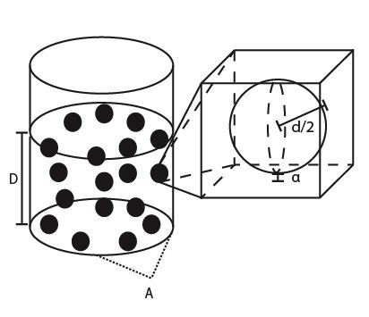
Figure 1: Schematic diagram of the biofilm structure. A cylindrical (or rectangular) container of depth, D, and cross-sectional area, A, holds the biofilm mass. Each bacterium occupies a spherical volume of diameter, d, corrected by a constant representing the space filled by surrounding EPS, α (see zoom-in).

Figure 2: Flow diagram indicating the interactions among the core components of the biofilm system. The total biofilm population, B_T, is divided into subpopulations (inside the rounded box). The phage particle population, P, directly interacts with only the subpopulation infected with latent phage, B_L.

Figure 3: Schematic diagram of the phage invasion process. Phage particles move into the biofilm structure via simple diffusion. Lysis of infected host cells in the phage-infested layer (indicated by a thickness of x) produces new pools of phage particles which undergo diffusion into the biofilm at rate, r_in, or out of biofilm at rate ,r_out. The depth of the biofilm structure is z.