Team:Peking/Modeling/CalculationProcess
From 2010.igem.org
(→Equations Set Up) |
|||
| Line 58: | Line 58: | ||
[[Image:Simple_network.png|center|50px]] | [[Image:Simple_network.png|center|50px]] | ||
<html> | <html> | ||
| - | <font size=1.5><br><b>Figure 4 simplest network</b> There is only one link from node A to node C and we don’t regulate the property of the link. Actually, whether it is activation, repression or no regulation is represented by | + | <font size=1.5><br><b>Figure 4 simplest network</b> There is only one link from node A to node C and we don’t regulate the property of the link. Actually, whether it is activation, repression or no regulation is represented by λ. |
<br></font> | <br></font> | ||
</html> | </html> | ||
Revision as of 13:04, 27 October 2010

Network Enumeration
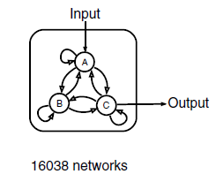
We use three nodes as a minimal framework: one node that receives input( A in Figure 2 ), a second node that transmits output( C in Figure 2 ), and a third node that can play diverse regulatory roles( B in Figure 2 ). There are 9 direct links among the three nodes and there are altogether 3^9=19,683 three-node topologies. With 3,645 topologies that have no direct or indirect links from the input to the output occluded, there remain a total of 16,038 possible three-node topologies that contain at least one direct or indirect causal link from the input node to the output node. For each topology, we sampled 10,000 sets of network parameters with the method of latin hypercube sampling (LHS, Figure 3). In all, we have analyzed a total of 16,038*10,000 different circuits. This search resulted in an exhaustive circuit function map used to extract core topological motifs essential for IOA.
Figure 2 Three-node network with all of its possible directed links(Ref. 7)
There are altogether 9 possible links and the input here is Hg(Ⅱ), and the concentration of C is taken as output.
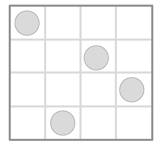
Figure 3 Latin Hypercube Sampling When sampling a function of N variables, the range of each variable is divided into M equally probable intervals, M sample points are then placed to satisfy the Latin Hypercube requirements. Then each sample is the Only one in each axis-aligned hyperplane containing it.
[TOP]Equations Set Up
Our model is based on mainly the following statements:
(1) The nodes are restricted to TF nodes so that the links stand for TF-TF interactions via DNA. The expression level is quantified by the equilibrium binding probability P of TF binding on its site and the maximum expression rate constant ![]() , and we adopt a constant
, and we adopt a constant ![]() to modify P to make different TFs equal status. When it comes to several TF factors, we use the multiplication of their
to modify P to make different TFs equal status. When it comes to several TF factors, we use the multiplication of their ![]() or
or ![]() to indicate their interactions.
to indicate their interactions.
(2) We take into consideration only the transcription and translation process because other reactions such as signal-transduction activities typically operate much faster and can be considered to be approximately at steady state on the slow timescales of transcription networks. Also the TF activity levels can be considered to be at steady state within the equations that describe network dynamics on the slow timescale of changes in protein levels. So that the equations contain only the accumulation and degradation of the protein products ( here the TFs).
(3) It has been observed that one ordinary gene usually has a nonzero expression level with no TFs on its binding site. We propose that one repressor will lower the initial expression level and one activator will shift it, further on, each TF has its unique contribution to the final expression level,that is, they shift or lower the expression level to different extents according to their own properties.
Consider first the simplest condition under which there is only one link from a node to another. (A![]() C, Figure 4)
C, Figure 4)
It is widely accepted that the possibility of TF binding to the binding site in promoter is (X*: the effective concentration of one TF; Kd : the dissociation constant )
According to hypothesis (1)&(3), the link from A(node1) to C(node3) can be translated as

( ![]() :the basal translation rate factor;
:the basal translation rate factor;![]() :the effective translation rate factor.)
:the effective translation rate factor.)
As  (Figure 5(a))
Thus  (Figure 5(b))(The subscript of X is the node number.)
Actually, the first component of the equation is the fundamental expression level of the network in which the ![]() is the possibility that the TF is off the DNA target site, and the second component of the equation is the effective expression level in which
is the possibility that the TF is off the DNA target site, and the second component of the equation is the effective expression level in which ![]() is the possibility that TF is on its site.
is the possibility that TF is on its site.
As to general conditions, there are

And in order to make the equations fit hypothesis 3,we deduced the proper range of ![]() , that is, no regulation
, that is, no regulation ![]() , activation
, activation  and repression
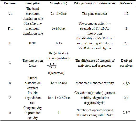
  .The choice of other Parameter values and their reference is in Table 1.
Figure 4 simplest network There is only one link from node A to node C and we don’t regulate the property of the link. Actually, whether it is activation, repression or no regulation is represented by λ.
Figure 5 MerR interacts with Hg(Ⅱ)& MerR-Hg binding to DNA (a)The orange poor arc sector stands for the MerR monomer and the orange major arc sector stands for the MerR dimer. The blue ball is Hg ion that can be bound by the MerR dimer, and only the complex can serve as Transcription Factor that promotes the expression of downstream genes. We list the balance equations, derive the calculation function of X* as above, and substitute this function to the ODE equations used in our model. (b) As the MerR dimer is only slightly repress DNA transcription, we regrad Kd' << K1*Kd, so neglecting the competitive binding of MerR dimer to DNA.
Table 1 Physiological range of the model parameters
[TOP]
Network Topologies’ Analysis
Aiming at getting the values of r for each circuit, we need to numerically simulate the ODE equations to get the steady-state concentration of output node C under each input concentration, and then making linear fit of input and output concentrations. As our input concentration range is 10-9~10-5, we select points that have the same logarithmic distance intervals, then simulate output evolution curve to get the steady concentration one point by one. We choose the fourth-order Runge-Kutta method to solve the ODE equations and so as to save calculation time, we adopt Implicit Runge-Kutta algorithm to get the output steady concentration when Input=10-9M and set the very concentration as initial value for the Newton-Raphson method for following different Input concentration. And considering the possibility of bistable network topology, we calculate the two directions (positive sequence and the reverse ) that Input concentration changes to avoid wrongly supposing it as one IOA function circuit.
[TOP]
 "
"


