Team:Peking/Modeling/Analysis
From 2010.igem.org
Evamonlight (Talk | contribs) (→Mechanisms of Minimal Semilog Networks and Key Parameters Analysis) |
Evamonlight (Talk | contribs) (→Mechanisms of Minimal Semilog Networks and Key Parameters Analysis) |
||
| Line 136: | Line 136: | ||
[[Image:SFunction21.png]] | [[Image:SFunction21.png]] | ||
<br><br> | <br><br> | ||
| - | When[[Image:SFunction31. | + | When[[Image:SFunction31.png]], there is<br><br> |
[[Image:SFunction41.png]],so: | [[Image:SFunction41.png]],so: | ||
<br><br> | <br><br> | ||
| Line 144: | Line 144: | ||
[[Image:SFunction71.png]] | [[Image:SFunction71.png]] | ||
<br><br> | <br><br> | ||
| - | Then we can see that the transform of | + | Then we can see that the transform of [[Image:0000.png]] fits well with the transform of the object function.<br> |
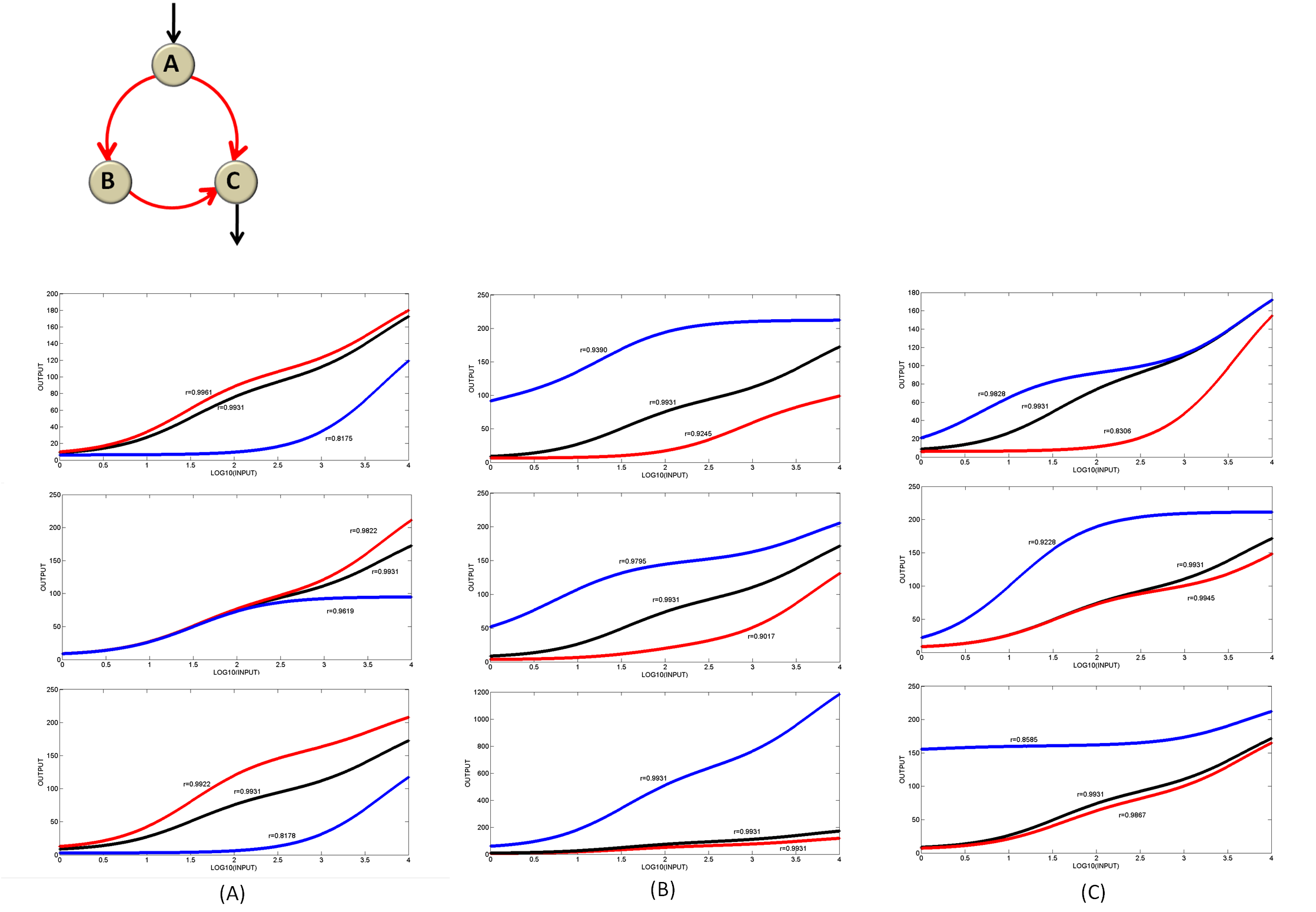
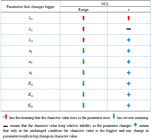
| - | Known the reason why the topology is functional in the object function, we need to analysis for the most important parameter in order to provide theoretical support for practice (Figure 16). We also list the parameter changes in Table 3. Among the nine parameters, the essential parameter for the output range is not obvious and that for r is the same condition – we can only see that [[Image:00.png]] has no influence on r. Based on an overall consideration, we suggest that in practice a smaller [[Image:004.png]] , a larger | + | Known the reason why the topology is functional in the object function, we need to analysis for the most important parameter in order to provide theoretical support for practice (Figure 16). We also list the parameter changes in Table 3. Among the nine parameters, the essential parameter for the output range is not obvious and that for r is the same condition – we can only see that [[Image:00.png]] has no influence on r. Based on an overall consideration, we suggest that in practice a smaller [[Image:004.png]] , a larger [[Image:000.png]] and a larger [[Image:00.png]] should be adopted. |
<br> | <br> | ||
[[Image:Semilog完整版.png|center|500px]] | [[Image:Semilog完整版.png|center|500px]] | ||
| - | <html><font size=1.5><b>Figure 16 Analysis for key parameters</b>We got all functional sets of parameters of AAN and selected randomly one set and processed it with Matlab to compare the differences once the parameters change. When analyzing one parameter, we only change this very parameter and keep others the same, and when we change the parameter to a lower level, we get the blue line, when to a higher level, we get the red line and the black line is for the unchanged parameter set. Each line has its Pearson Correlation Coefficient r marked in the figure. The X Axis is the concentration of Hg ion as INPUT whose range is 1 to 10000 nM, and the Y Axis is the concentration of node C with the unit of nM. (A) We analyze | + | <html><font size=1.5><b>Figure 16 Analysis for key parameters</b>We got all functional sets of parameters of AAN and selected randomly one set and processed it with Matlab to compare the differences once the parameters change. When analyzing one parameter, we only change this very parameter and keep others the same, and when we change the parameter to a lower level, we get the blue line, when to a higher level, we get the red line and the black line is for the unchanged parameter set. Each line has its Pearson Correlation Coefficient r marked in the figure. The X Axis is the concentration of Hg ion as INPUT whose range is 1 to 10000 nM, and the Y Axis is the concentration of node C with the unit of nM. (A) We analyze [[Image:000.png]] [[Image:00.png]] [[Image:00000.png]]from top to bottom. (B) the degradation rate of node A , B and C, respectively,[[Image:002.png]][[Image:003.png]][[Image:004.png]](C) The dissociation rate for each link:[[Image:008.png]][[Image:005.png]][[Image:009.png]].<br></font></html> |
<br> | <br> | ||
<html><font size=1.5><b> Table 3 The change of two important characters as the parameters rise</b></font></html> | <html><font size=1.5><b> Table 3 The change of two important characters as the parameters rise</b></font></html> | ||
Revision as of 04:14, 27 October 2010

Analyses and Results
Contents |
IOA Network Analysis
We get the value of the characters (r mainly) after calculation under each set of parameters, then we analyse them trying to find one simple topology that can function well.
Identifying Minimal IOA Networks
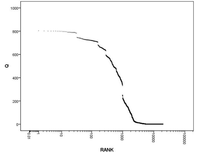
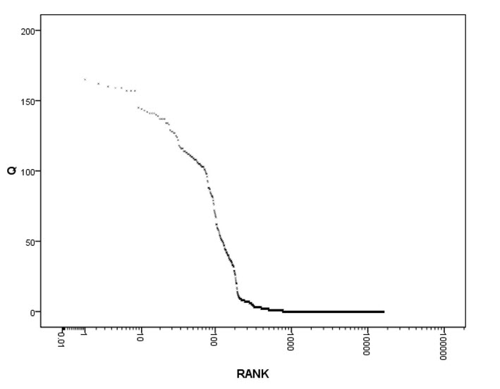
Here we define Q value as the number of IOA function circuit among 10000 sets of network parameters, and it indicates the robustness of one topology to finish the IOA function—the larger Q value is, the more robust the topology is. We sort in reverse sequence all the network topologies according to their Q value and the x axis is their rank( Figure 6).We can observe that most network topologies have 0 or low Q value while there’s only a small part of the topologies having large Q value.
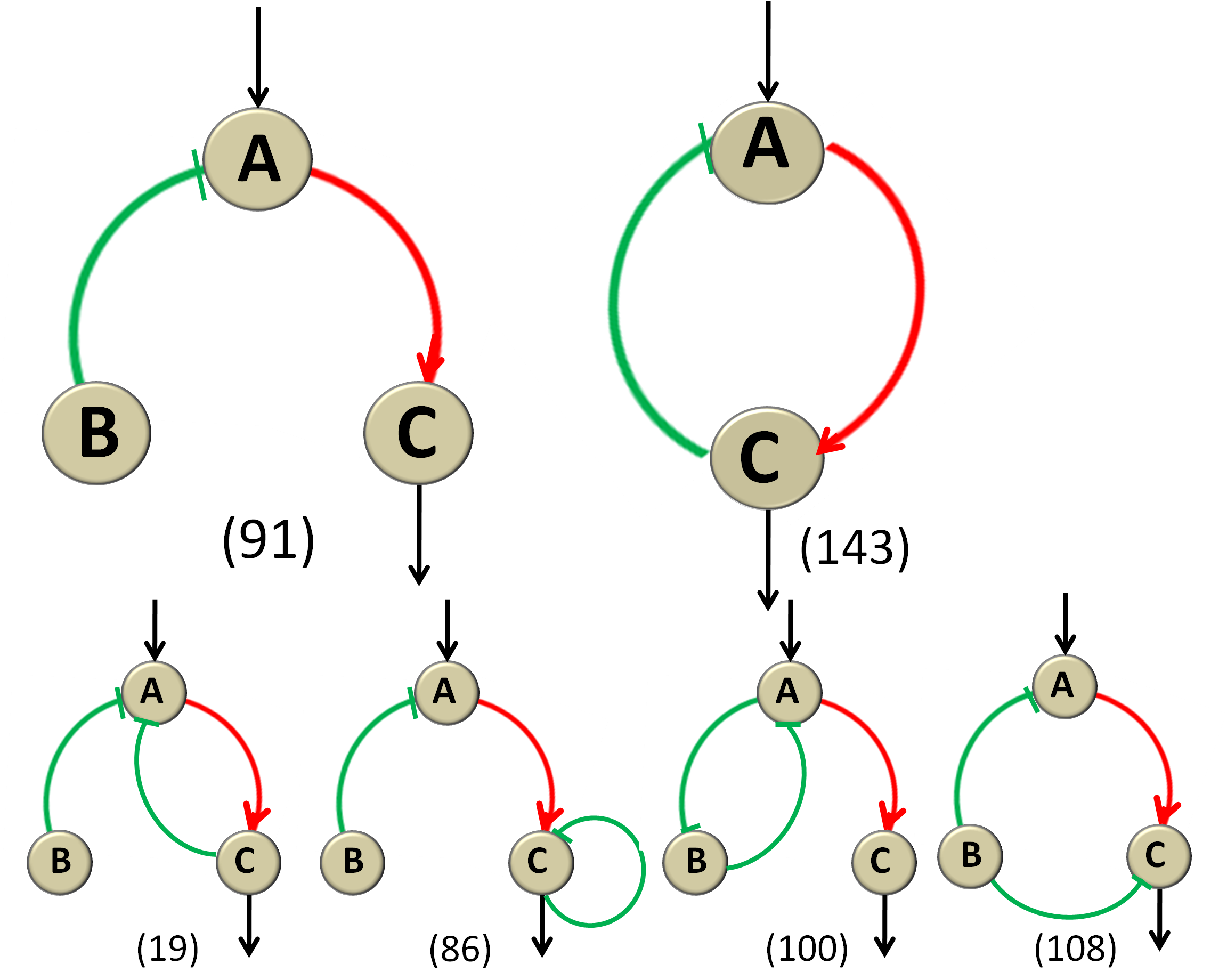
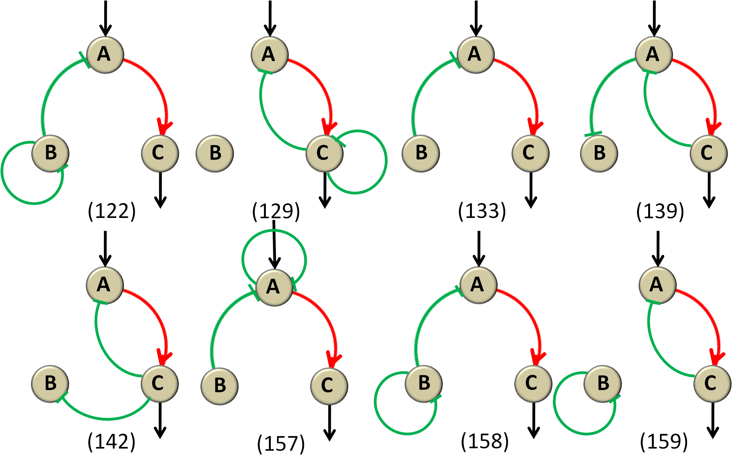
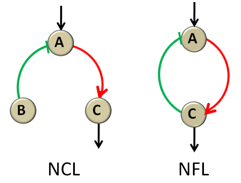
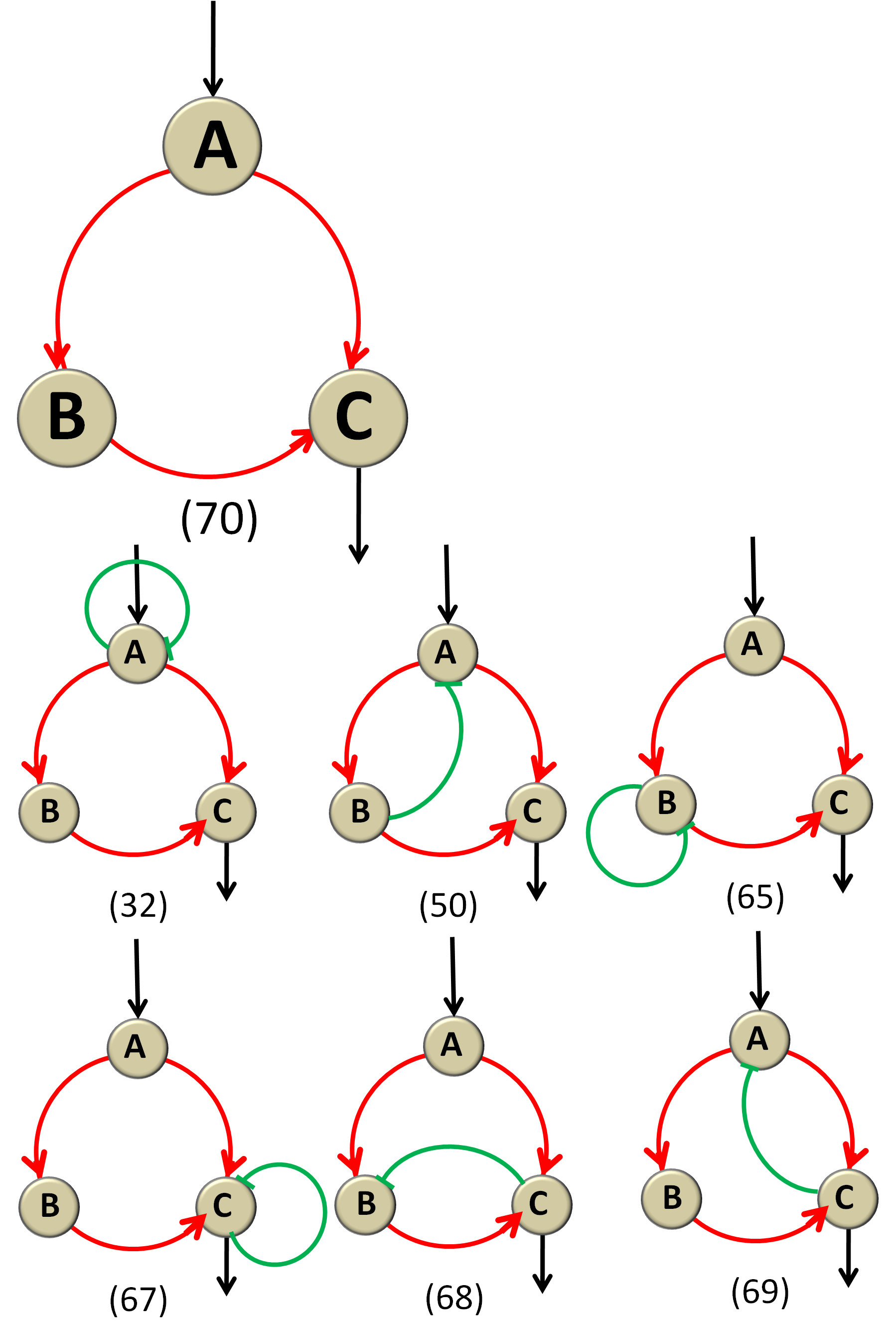
We firstly analysis the first 160 network topologies ( Q >=705 ) and list in Figure 7 all the simplest topologies that have only 3 or less direct links between the three nodes.( Figure 7) Among the 14 topologies, there are 12 three-link networks and 2 two-node networks so that we can see that the minimal number of links for the topologies to be functional is two but the most usual number is 13. The common features of the networks capable of IOA are either one negative control loop (NCL) or one negative feedback loop (NFL). Here we define NCL as a topology that has one negative control on the input-receiving node (A) from the intermediate node (B) and one positive regulation on the output node (C) from A node.(as the 1st topology in Figure 7 and the 1st one in Figure 8) Similarly we define NFL as a topology that share the positive-regulation link from A to C, while uniquely have one negative feedback from C to A.(as the 2nd topology in Figure 7 and the 2nd one in Figure 8) And the NCL topology seemingly more robust than the NFL topology, as there are 9 topologies out of the 14 simplest networks contain NCL topology compared to 6 of NFL, so that B node appears to be important, which will be discussed in details in the following part.
Figure 6 The Q value network topologies SequenceWe sort in reverse sequence all the network topologies according to their Q value. X Axis is their ranks, while Y Axis is their corresponding Q values. The figure indicates that most network topologies have 0 or low Q value while there’s only a small part of the topologies having large Q value.
Figure 7 All Functional NetworksThe numbers below each network are their ranks. The two bigger topologies have 2 links while the other 12 networks have 3 links. In each network, the green arc with one short straight line at one end stands for repression from the start node to the end node and the red arc with one arrow at one end stands for activation.
Figure 8 The NCL and NFL topologyThe green and red line have the same meaning as in Figure 7.
[TOP]
Mechanisms of Minimal IOA Networks and Key Parameters Analysis
Aimed at answering the question why the two topologies defined above (Figure 8) is functional in IOA, we unravel their mechanisms using the ODE equations in this part, also getting the parameter restrictions of each topology.
NCL Topology
When the network has built steady state:
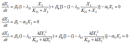
Solve the equations:
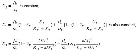
If there is ![]() , then
, then
![]()
Because X1 is constant, the coefficient of I is also constant. So there comes the linear correlation between X3(output concentration) and I.
When ![]() ,
,
![]()
And the concentration of B node is actually part of the slope coefficient the linear equation, we can imagine that the function of B node is to lower the concentration of A straightly without the interference of other factors as well as control the concentration of A more precisely and more freely to make the parameter restriction easier to achieve and at the same time the output range is not too small. As we know, the stochastic error may make vague the linear relationship when the values of y axis are too near. The lower concentration X2 is, the steeper the line is, and so the bigger the range is, which in biology means that the bioreporter is more sensitive to certain environmental signal. Through modifying the parameters of node B, we can get a proper concentration of A node to achieve a good r. In all, the node B is a proportion node.
NFL Topology

Also solve the equations:

If![]() ,then
,then![]() is constant;
is constant;
And if![]() ,then
,then![]() ,which correlation is the same as the NCL Topology.
,which correlation is the same as the NCL Topology.
Compare X1 here with the concentration of node A in NCL topology, one can easily discover that X1 here is higher and more dull, which makes it more hard to get a balance between satisfying the second parameter restriction and the need for the range to be rational. Then we can understand why NFL topology is less than NCL in high-Q-value topologies.
Key Parameter Analysis
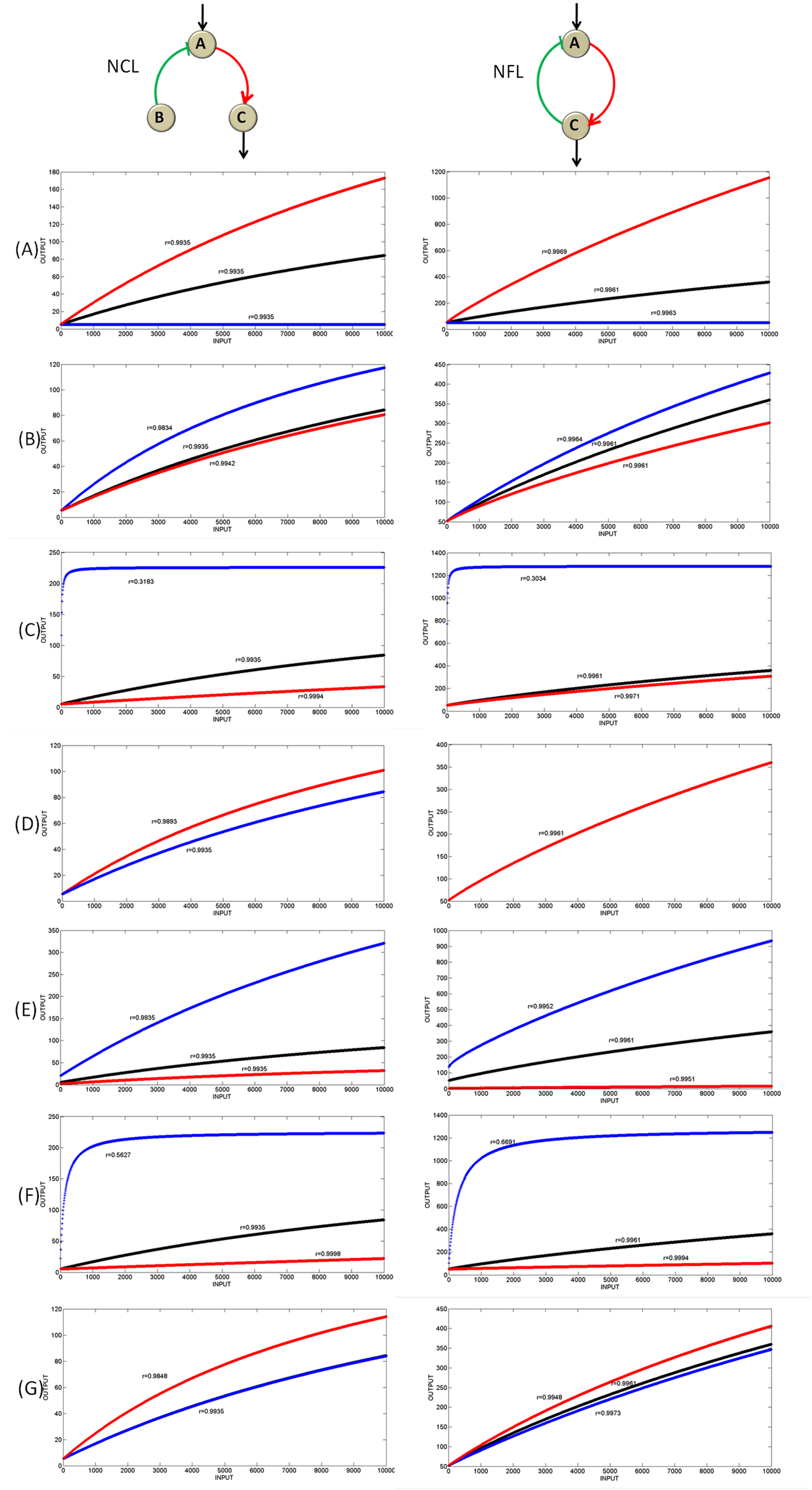
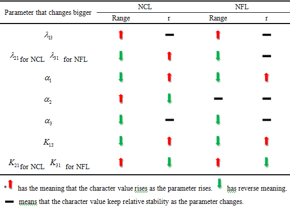
Aimed at unraveling the relative importance among parameters, we got all functional sets of parameters of NCL&NFL and selected randomly one set, respectively, from the two topologies and processed them with Matlab to compare the differences once the parameters change. The results are in Figure 9. From changes of the two important characters – the output range and r with the change of parameters (Table 2), we got the answer to previous questions.
Figure 9 Analysis for key parametersWe got all functional sets of parameters of NCL&NFL and selected randomly one set, respectively, from the two topologies and processed them with Matlab to compare the differences once the parameters change. When analyzing one parameter, we only change this very parameter and keep others the same, and when we change the parameter to a lower level, we get the blue line, when to a higher level, we get the red line and the black line is for the unchanged parameter set. Each line has its Pearson Correlation Coefficient r marked in the figure. The X Axis is the concentration of Hg ion as INPUT whose range is 1 to 10000 nM, and the Y Axis is the concentration of node C with the unit of nM.(A) We analyze  for both topologies. (B)
 for NCL and
 for NFL (C) The degradation rate of A (
 )for both topologies (D) The degradation rate of B(
  )for both (E)The degradation rate of C(
 ) for both (F) The dissociation rate of A to the binding site on the gene of C(
  ) for both (G)
 for NCL and
 for NFL.
For NCL, the degradation rate of A (![]() ) and the value of Kd from node A to node C (
) and the value of Kd from node A to node C ( ![]() ) are relatively more important to r, and the degradation rate of C (
) are relatively more important to r, and the degradation rate of C (![]() ) along with Kd from node A to node C (
) along with Kd from node A to node C ( ![]() ) are essential to the output range, while the constant indicating repression from B to A(
) are essential to the output range, while the constant indicating repression from B to A(![]() ) , the degradation rate of B (
) , the degradation rate of B (![]() ) as well as Kd from node B to node A (
) as well as Kd from node B to node A (![]() ) influence little both characters. From Table 2 and the analysis above, we can draw the conclusion that in practice, the parameter
) influence little both characters. From Table 2 and the analysis above, we can draw the conclusion that in practice, the parameter ![]() should be larger and
should be larger and ![]() should be as small as possible. While for NFL, the condition is similar. It is still
should be as small as possible. While for NFL, the condition is similar. It is still ![]() and
and ![]() that are important to r, but the key parameters on the output range are
that are important to r, but the key parameters on the output range are ![]()
![]()
![]()
![]() , more than the key parameters for output range for NCL. So the suggest to practice is still smaller
, more than the key parameters for output range for NCL. So the suggest to practice is still smaller ![]() and larger
and larger ![]() , what’s more, there should be smaller
, what’s more, there should be smaller ![]() for larger output range according to the character changes in Table 2.
for larger output range according to the character changes in Table 2.
Table 2 The change of two important characters as the parameters rise
[TOP]
Parameters Tendency of the IOA Networks
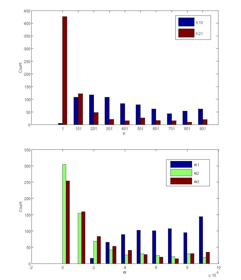
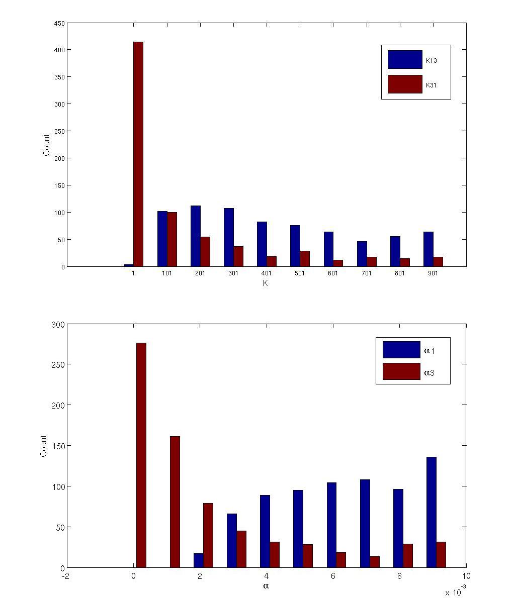
In order to test the correctness of our analysis about the key parameters, we look more closely at the parameters of the simplest IOA networks. For the two simplest networks in Figure 6, we examine the distribution of the parameter values which can realize linear response between input and output out of the total 10000 sets of parameters used in the search.(Figure10, Figure11)
It can be seen that the constant K of the repression (K21 and K31) are generally lower compared to K13, which means that there should be an intense repression on node A. Such a result also fits well with the condition![]() used in the derivation above.
used in the derivation above.
We also notice that the degradation rates, α, of the nodes also show apparent tendency. The degradation rate of the node A is generally higher, while the repressing nodes (B or C) have lower degradation rates. Such a tendency also shows that the repression on node A should be intense in order to establish a more linear response curve between input and output.
[TOP]
Analysis of All Possible Three-Node Networks
The above analyses focused on minimal( less than or equal to 3 links) three-node networks and identified simple topologies that are sufficient for IOA function, also unraveling the mechanism that the topologies work. But whether the topologies are necessary for the IOA function is not understood yet. In other words, are the identified minimal topologies the foundation of all possible networks, or are there more complex higher-order solutions that do not contain these minimal topologies? To answer the questions above, we analysis the first 160 topologies (Q>705) that are well capable of the IOA function.(Figure 12)
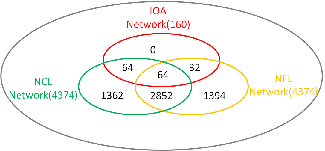
Figure 12 Analysis of the first 160 networks We count all the NCLs and NFLs and also the IOA networks, and discover that all of the IOA networks can be classified into NCL/NFL/the combination of the two. And there are more IOA functional network featured in NCL than those characterized with NFL.
Analysis of these robust topologies shows that they are overrepresented with NCL and NFL. All 160 topologies contain at least one NCL or NFL motif ( or both ). These results indicate that at least one of these motifs is necessary for IOA function.
Supplementarily, the NCL average Q value(AQV)of all 19683 topologies is 17.14 while the NFL AQV is only 9.36, which again indicate that the NCL is more robust than NFL that have drew conclusion in the minimal topology analysis.
[TOP]
Motif Combinations that Improve IOA
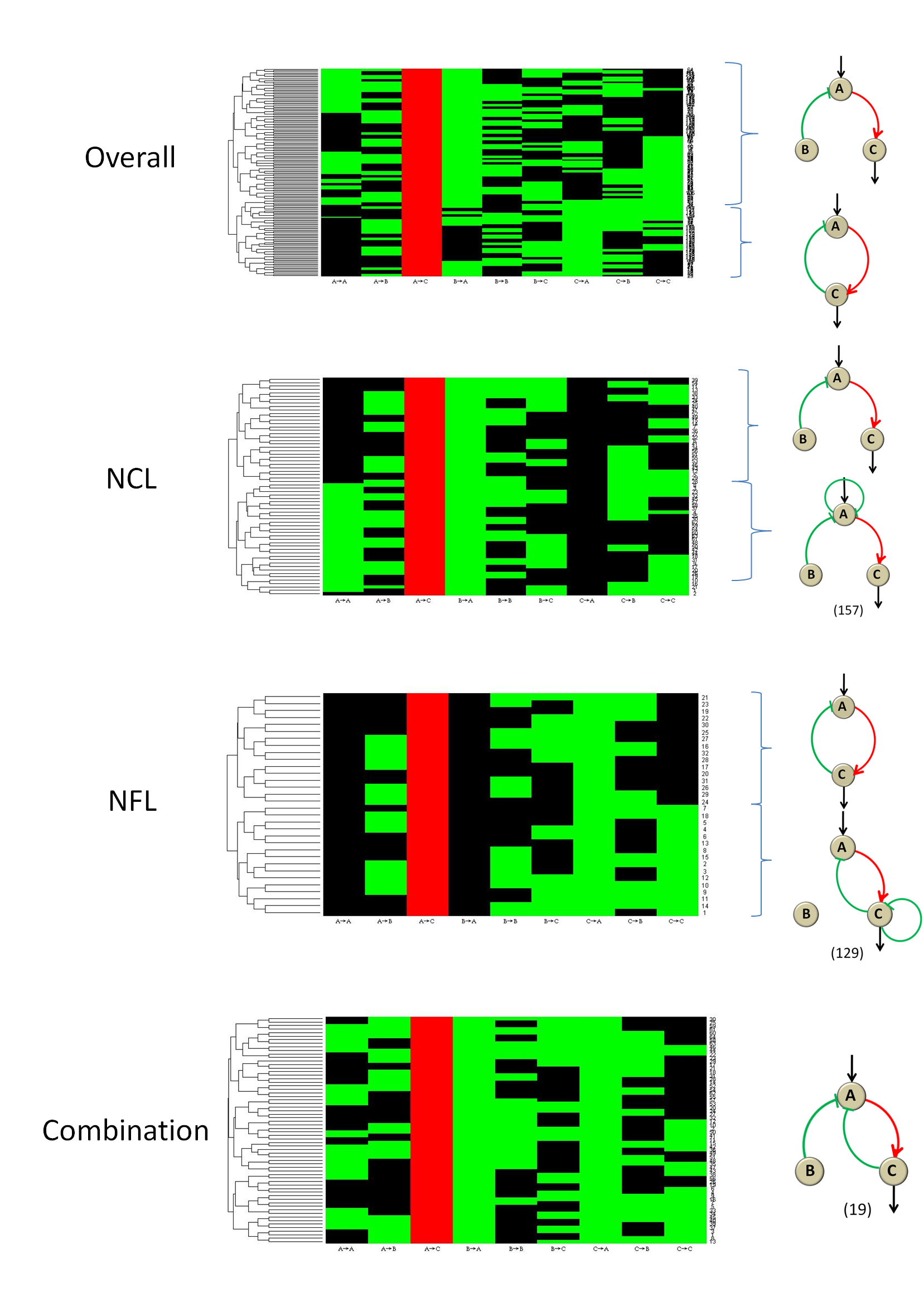
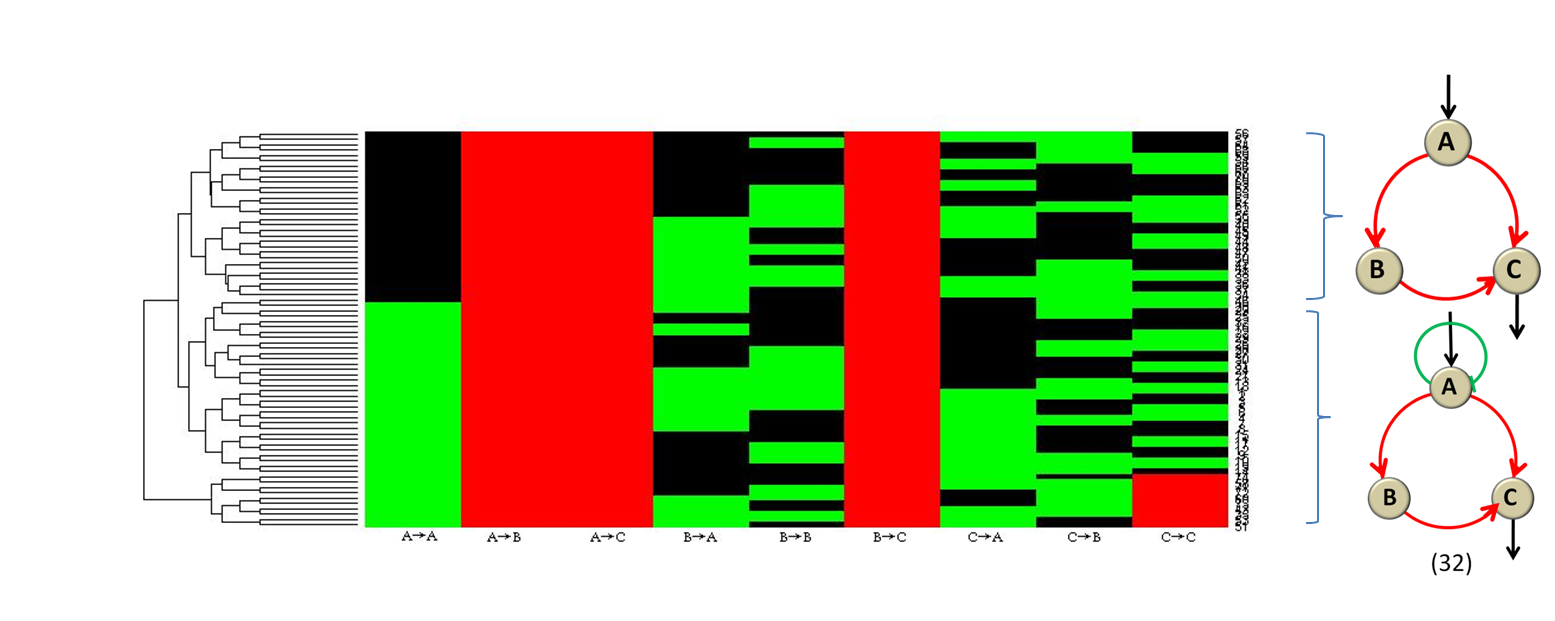
To investigate what additional features can improve the functional performance in some more complex and more robust networks than minimal topologies, we clustered the first 160 networks and then cluster them respectively in three categories: NCL, NFL and the combination of the two. (Figure 13)
Figure 13 The clustergrams of the networksWe use the clustergram command in matlab to get the additional features of the functional networks. The nine vertical rectangle bar stand for nine links in Figure 2 which are, respectively, from A to A, from A to B, from A to C, from B to A, from B to B, from B to C, from C to A, from C to B, from C to C. And red stands for activation, green for repression and black for no regulation. The topologies on the right are corresponding minimal topologies that is shown in the clustergrams on the left.
The results clearly indicate that apart from the link from A to C, there should be no positive regulation, and the NFL topology hates the link from A to A, while the combination topologies show no additional tendency.
[TOP]
Summary
In all, by exhaustively searching all network and analyzing the results, we draw the conclusion that NCL meets our need in application well, and we get the proper parameter range for practice.
[TOP]
More Advanced Model
As the IOA function still cannot work well to ensure the linear relationship when the input range spans several orders of magnitude, we search for semilog networks further using the same method. Semilog represents that the output and LOG(input) fit linear relationship, different from IOA in x axis in Figure 1.
Identifying Minimal Semilog Networks
We again get the Q-Rank Figure. Topologies that have large Q value are still the minority.
Listed in Figure 15 are all the simplest topologies whose Q value is above 100 that have 4 or less direct links between the three nodes.( Figure 2) There are only one 3-link topology( as the 7th topology in Figure 2) out of all the 7 simplest topologies, and it has exactly the common features of the seven topologies: two positive controls from A node to respectively B node and C node, and one positive control from B to C. We call it the All Activated Network(AAN). The role of different nodes and links will be discussed in the next part.
Figure 14 The Q value network topologies SequenceWe sort in reverse sequence all the network topologies according to their Q value. X Axis is their ranks, while Y Axis is their corresponding Q values.
Figure 15 All Functional NetworksThe numbers below each network are their ranks. The bigger topology has 2 links while the other 6 networks have 3 links. In each network, the green arc with one short straight line at one end stands for repression from the start node to the end node and the red arc with one arrow at one end stands for activation.
[TOP]
Mechanisms of Minimal Semilog Networks and Key Parameters Analysis
In order to unravel the mechanism that AAN functions, we analysis the topology with the ODE equations, and we also get the key parameters in this part.
When the network reaches its steady state,

Solve the equations,

When![]() , there is
, there is
![]() ,so:
,so:

As to the object function![]() , we adopt the method of Taylor expansion
, we adopt the method of Taylor expansion
![]()
Then we can see that the transform of ![]() fits well with the transform of the object function.
fits well with the transform of the object function.
Known the reason why the topology is functional in the object function, we need to analysis for the most important parameter in order to provide theoretical support for practice (Figure 16). We also list the parameter changes in Table 3. Among the nine parameters, the essential parameter for the output range is not obvious and that for r is the same condition – we can only see that ![]() has no influence on r. Based on an overall consideration, we suggest that in practice a smaller
has no influence on r. Based on an overall consideration, we suggest that in practice a smaller ![]() , a larger
, a larger ![]() and a larger
and a larger ![]() should be adopted.
should be adopted.
Figure 16 Analysis for key parametersWe got all functional sets of parameters of AAN and selected randomly one set and processed it with Matlab to compare the differences once the parameters change. When analyzing one parameter, we only change this very parameter and keep others the same, and when we change the parameter to a lower level, we get the blue line, when to a higher level, we get the red line and the black line is for the unchanged parameter set. Each line has its Pearson Correlation Coefficient r marked in the figure. The X Axis is the concentration of Hg ion as INPUT whose range is 1 to 10000 nM, and the Y Axis is the concentration of node C with the unit of nM. (A) We analyze [[Image:000.png]] [[Image:00.png]] [[Image:00000.png]]from top to bottom. (B) the degradation rate of node A , B and C, respectively,[[Image:002.png]][[Image:003.png]][[Image:004.png]](C) The dissociation rate for each link:[[Image:008.png]][[Image:005.png]][[Image:009.png]].
Table 3 The change of two important characters as the parameters rise
[TOP]
Parameters Tendency of the Semilog Networks
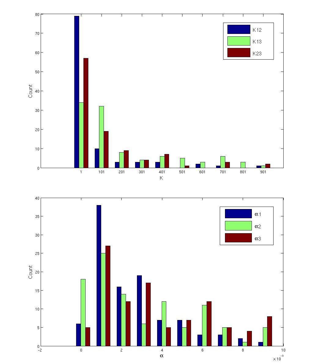
It can be seen from the distribution of K and α values that compared to networks with linear response curve, single parameter shows much less tendency. Instead, to establish a semi-log response curve may require the cooperation of multiple parameter values.
[TOP]
Analysis of All Possible Three-Node Networks
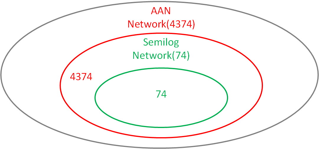
Again through the analyses above, we only know that AAN can be functional in Semilog function, but whether the topology is necessary among the more complex networks are still unknown, so we analysis all of the first 74 topologies (Q>100) that are well capable of the Semilog function.(Figure 18)
Figure 18 Analysis of the first 160 networks We count all ANNs and the Semilog networks whose Q value is above 100, and discover that all of the Semilog networks are make up of the ANN topology and the topologies contain it.
Analysis of these robust topologies shows that they all contain AAN, so that the very topology is necessary for Semilog function.
[TOP]
Motif Combinations that Improve Semilog Linear
To investigate what additional features can improve the functional performance in some more complex and more robust networks than minimal topologies, we clustered the first 74 networks.(Figure 19)
Figure 19 The clustergrams of the networksWe use the clustergram command in matlab to get the additional features of the functional networks. The nine vertical rectangle bar stand for nine links in Figure 2 which are, respectively, from A to A, from A to B, from A to C, from B to A, from B to B, from B to C, from C to A, from C to B, from C to C. And red stands for activation, green for repression and black for no regulation. The topologies on the right are corresponding minimal topologies that is shown in the clustergrams on the left.
The results clearly indicate that apart from the link from A to B, from A to C, from B to C, and from C to C, there should be no positive regulation.
[TOP]
Advandced Part Summary
Hence, we finally get the practical form of genetic circuits that can be adopted by our wetlab part. And the mechaism and parameter preferences are understood to some extent.
[TOP]
 "
"
