"

From 2010.igem.org

Revision as of 07:39, 27 October 2010 (view source) Ddbuckley (Talk | contribs) (→Model 1) ← Older edit		Latest revision as of 02:36, 28 October 2010 (view source) Ricky (Talk | contribs) (→Kinetic modelling of the ethylene generator)
(50 intermediate revisions not shown)
Line 4:		Line 4:
	== Introduction ==		== Introduction ==
-	[[Image:Monash_Australia_Yang-cycle.png|200px|thumb|left|Yang cycle]]	+	[[Image:Monash_Australia_Yang-cycle.png|200px|thumb|left|Figure 1: Yang cycle. In red - the reaction we wish to model ''in silico''.]]
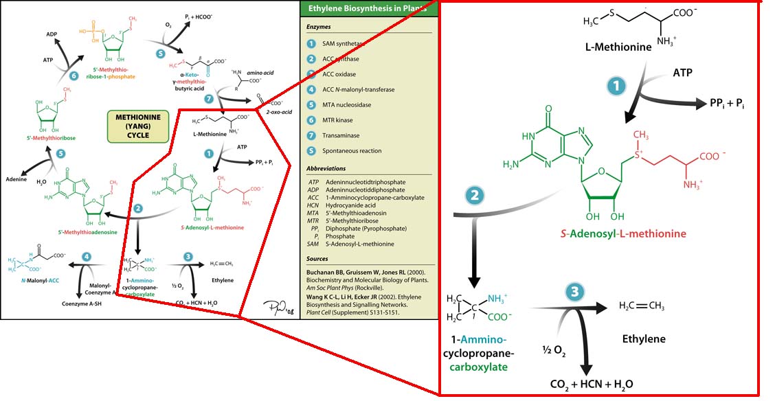
-	The three key enzymes we require are highlighted in the image, <b>SAM synthase</b>, <b>ACC synthase</b> and <b>ACC oxidase</b>. SAM synthase converts methionine into S-Adenosyl-L-Methionine (SAM), using ATP for an adensoyl group. The second step involves ACC synthase, which cleaves the amino butyrate from SAM, releasing 1-aminocyclopropane-1-carboxylic acid (ACC). Released ACC is then processed by ACC Oxidase which converts ACC to ethylene by cleaving the carboxylic acid off as carbon dioxide and its neighboring carbon with the amino group as cyanide gas. By using such a system to produce ethyene gas we can potentially reduce costs involved with current production methods by reducing temperature requirements by 30 fold.	+	The three key enzymes we require are outlined in the image Figure 1 (left), <b>SAM synthase</b>, <b>ACC synthase</b> and <b>ACC oxidase</b>. SAM synthase converts methionine into S-Adenosyl-L-Methionine (SAM), using ATP for an adensoyl group. The second step involves ACC synthase, which cleaves the amino butyrate from SAM, releasing 1-aminocyclopropane-1-carboxylic acid (ACC). Released ACC is then processed by ACC Oxidase which converts ACC to ethylene by cleaving the carboxylic acid off as carbon dioxide and its neighboring carbon with the amino group as cyanide gas. By using such a system to produce ethyene gas we can potentially reduce costs involved with current production methods by reducing temperature requirements by 30 fold.
	== Kinetic modelling of the ethylene generator ==		== Kinetic modelling of the ethylene generator ==
-	The program tinkercell was used to model the synthesis of ethylene in our e.coli cell. Where, in addition to the qualitative representation (figure 1) the program allowed, simulation of the model could be exercised inorder to measure the flux of metabolites – with respect to time - in the system given the input of values pertaining to substrate/enzyme concentration, and reaction rates were inputted. In addition to experimental data, with a model, theoretical data can be obtained using the model to extrapolate quantitative data corresponding to mRNA, protein and ethylene outputs under set parameters and assumptions in silico. As a result, using the given theoretical model outputs as a benchmark, manipulations to the parameters and assumptions set can be made in vitro/in vivo in order to achieve higher outputs in future studies of the 'ethylene generator'.	+	The program tinkercell was used to model the synthesis of ethylene in our E.coli cells. Where, in addition to the qualitative representation (figure 2 & 4) the program allowed, simulation of the model could be exercised inorder to measure the flux of metabolites – with respect to time - in the system given the input of values pertaining to substrate/enzyme concentration, and reaction rates were inputted. Figure 2 or Model 1 was designed to include fixed concentrations at a steady state ratio of 1:1:1. This design ensured sensible approximate values of ethylene output were obtained given the correctness of enzyme rates and other parameters used.
-	==<H2> Aims of the Kinetic Modelling </H2>==	+
		+	Adapting on to model 1, quantitative data in silico corresponding to mRNA transcription, protein translation,  and degradation were implimented into a more complex design - giving model 2. As a result, more realistic outputs of ethylene could be found. This design could then be used to compare and contrast actual ethylene values obtained experimentally. Hence the effiency of our E.coli cells could then be calculated. Depending on the effiency value, certain factors and variables could be changed in order to attempt to reach our tinkercell output.
		+
		+	The benefit of using Tinkercell to better understand our system, subsequently also allows us to distinguish the practicality of our project. That is, for example, if low levels of ethylene were predicted to be produced from the model at certain parameters, then efforts into favouring and adapting our system as a plant signalling/communication system could be aimed for in reality under those sorts of conditions. In contrast, if ethylene production was indicated by the model to be high for example, then again, under those certain set of parameters efforts could be re-directed into shaping the objective of the system to be used for plastic production. Hence, by modelling our project using Tinkercell, direction into where the project may lead to in the future can be better defined.
		+
		+	==<H2> Objectives </H2>==
	-To determine the maximum output of ethylene <p> </p>		-To determine the maximum output of ethylene <p> </p>
Line 22:		Line 27:
	<H4> Introduction to Model 1 </H4>		<H4> Introduction to Model 1 </H4>
-	[[Image:Cell12.jpg|200px|thumb|left|Model 1]]	+	[[Image:Cell12.jpg|300px|thumb|left|Figure 2: A visual construction of Model 1 using ''Tinkercell'']]
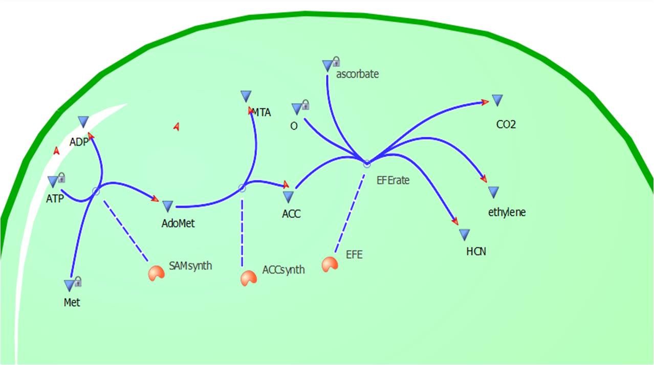
-	This model was designed to be the starting point of the our kinetic modelling. Therefore it was decided to begin with a realitivly simple construct.This uncomplicated system could then be used to obtain an ethylene output. This design comprised only of three enzymes and lacked the transcription and translation stages. The enzymes invloved were SAM synthetase, ACC synthase and ACC oxidase or EFE (ethylene forming enzyme). These enzymes were presnt at fixed concentrations (10, 100, 1000 and 3000 uM) and in the 1:1:1 ratio.. This ensured that the model was plain yet ultimately obtained a resonable yet simple ethylene output. Therefore with fixed enzyme concentrations the rate at which ethylene is produced depends on the Vmax of the specific enzymes.	+	This relatively simple model - as represented in figure 2 - was designed to be the starting point of our kinetic modelling. This uncomplicated system could then be used to obtain an ethylene output. This design comprised only of three enzymes and lacked the transcription and translation stages. The enzymes involved were SAM synthetase, ACC synthase and ACC oxidase - also known as EFE (ethylene forming enzyme). These enzymes were present at fixed concentrations (10, 100, 1000 and 3000 uM) and in a 1:1:1 ratio. Although basic, this model in essence was able to give reasonable output values for ethylene produced. Furthermore with fixed enzyme concentrations the rate at which ethylene is produced depends on the Vmax of the specific enzymes.
-	This specific rate is defined by the Michaelis-Menton Equation	+
		+
		+
		+	This specific rate is defined by the Michaelis-Menton Equation:
Line 35:		Line 43:
	<H4>Assumptions for Model 1</H4>		<H4>Assumptions for Model 1</H4>
-	- A 1:1:1 steady state of enzymes <p> </p>	+	- A 1:1:1 steady state of enzymes. <p> </p>
-	- No production inhibition <p> </p>	+	- No product inhibition. <p> </p>
-	-Substrates (ATP, L-Methionine etc) kept at a constant value due to homeostatic mecahnisms in E.coli <p> </p>	+	-Substrates (ATP, L-Methionine etc) kept at a constant value due to homeostatic mechanisms in E.coli. <p> </p>
-	- The best value (km, kcat etc) was always chosen to ensure maxiumum yield of ethylene <p> </p>	+	- The best value (km, kcat etc) was always chosen to ensure maximum yield of ethylene. <p> </p>
	----		----
Line 51:		Line 59:
	<b>SAMsynth Km(Met)</b>- 92 uM<p> </p>		<b>SAMsynth Km(Met)</b>- 92 uM<p> </p>
-	<b>ACCsynth Km(AdoMet)</b>- 37 uM <p> </p>	+	<b>ACCsynth Km(AdoMet/SAM)</b>- 37 uM <p> </p>
	<b>EFE Km(ACC)</b>- 12 uM <p> </p>		<b>EFE Km(ACC)</b>- 12 uM <p> </p>
Line 64:		Line 72:
	-----		-----
	<H4> Graphs and results</H4>		<H4> Graphs and results</H4>
-	[[Image:graph1.jpg|300px|thumb|left|EThylene Production at different steady state concentration]]	+	[[Image:graph1.jpg|300px|thumb|left|Figure 3: Ethylene Production at different steady state concentration]]
-	An explanation of this Graph	+	Using Tinkercell a graphical representation of 'Model 1' was generated (Figure 3) using deterministic stimulation.
		+	In this figure a graphical representation of the rates - generated internally by Tinkercell's mathematical alogarithms - of ethylene production are shown for each fixed enzyme concentration assumed.
		+	As a result not only is production of ethylene shown to be increasing linearly with time, but at a greater rate with increasing concentration of enzyme (SAM synthetase, ACC synthase, EFE) used.
		+
		+
		+
		+
		+
		+
		+
		+
		+
		+
		+
		+
		+
		+
		+	-
	== <H2>Model 2</H2>==		== <H2>Model 2</H2>==
-	[[Image:Monash_modeling.png|200px|thumb|left|Figure 1: Model 2]]	+	[[Image:Monash_modeling.png|300px|thumb|left|Figure 4: A visual construction of Model 2 using ''Tinkercell'', where transcription and translation are taken into account ]]
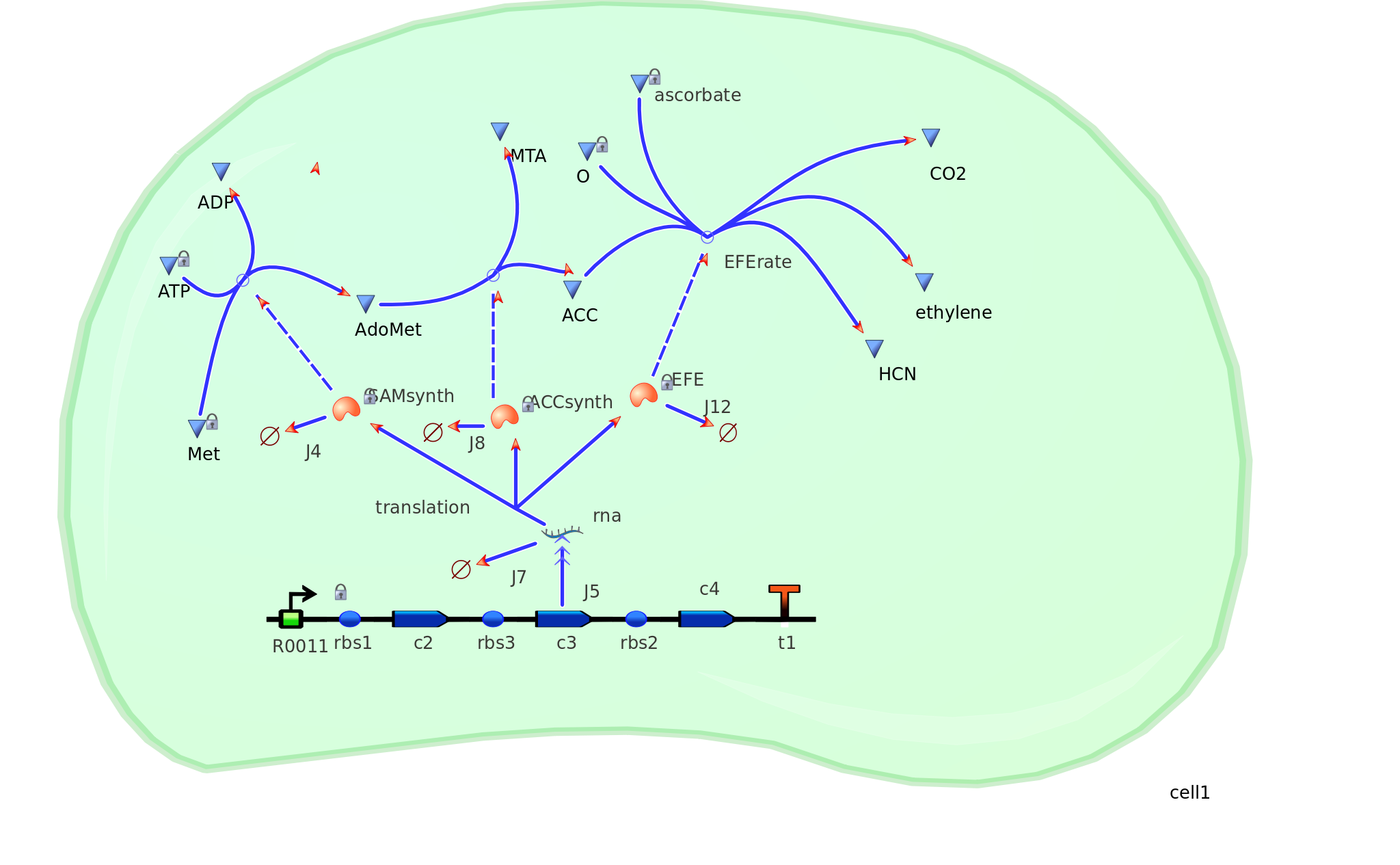
-	Model 2 explores the more complicated version of our kinetic modelling. It aims to incorporate the transcription and translation rates of the cell into the final design. This calculation begins to become more difficult due to problomatic degredation,transcription and translation rates. However these values where obtained from the [http://www.ebi.ac.uk/biomodels-main/BIOMD0000000012 Elowitz repressilator model]. Of the many sources browsed it was determined that this source seemed to be the most accurate and hence its values were used. Therefore the transcription and translation rates of mRNA and proteins constantly changes the final concentration of the three enzymes. This changing concentration of enzymes then produces ethylene at a more reliable rate. Therefore this model is designed to produce a more accurate representation of the ethylene producing biological pathway	+	Model 2 explores the more complicated adaptation of model 1 by incorporating the transcription, translation, and degradation rates of protein and mRNA into the final design. As a result a more realistic model of what would really be happening in the cell leading to ethylene production could be achieved. Of all the sources studied, it was decided that values from the [http://www.ebi.ac.uk/biomodels-main/BIOMD0000000012 Elowitz repressilator model] would be most sensible and relevant to our system. Therefore the degradation, transcription and translation rates were adapted from this model onto ours to factor in fluctuations in concentrations of our three enzymes, as unlike in model 1, enzyme concentration would not realistically be in a 1:1:1 ratio. Therefore using these values, model 2 was able to more realistically follow the metabolic pathway of ethylene production where fluctuations in enzyme concentration were taken into consideration – rather than having them fixed as in model 1.
-	-----	+
		+
		+
		+
		+
		+
		+
		+
		+
		+
		+
		+	-------
	<H3> Elowitz Degradation Values </H3>		<H3> Elowitz Degradation Values </H3>
Line 84:		Line 120:
	-----		-----
	<H3> Graphs and results </H3>		<H3> Graphs and results </H3>
-	more to come	+	[[Image:Mrnagraph.png|300px|thumb|left|Figure 5: Production of mRNA in the cell]] The rate at which mRNA is produced can be seen to start off at a rapid rate. However as time goes on the mRNA can be seen to reach a steady state.<p></p>
		+
		+
		+
		+
		+
		+
		+
		+
		+
		+
		+
		+
		+
		+
		+
		+
		+
		+
		+
		+
		+
		+
		+
		+
		+
		+
		+	[[Image:Enzymegraph.png|300px|thumb|left|Figure 6: Production rate of the three different enzymes]] Due to the polycystronic translation of the mRNA all the three enzymes are produced in a 1:1:1 ratio. To begin the enzymes are produced at a realitively fast rate however as time proceeds they fail to reach a steady state. In E.coli it is known that all enzymes eventually reach a steady state otherwise energy and resources would be depleated. Hence this graph suggests plausibility for approximately the first 10 seconds of production; sfter that the data looks unrealistic and implausible in an E.coli cell.
		+
		+
-	== Construct --> mRNA --> enzymes (SAMsynth, ACCS, EFE) ==
-	[[Image:tran.jpg|200px|thumb|left|]]
-	== Met --> SAM (AdoMet) ==
-	[[Image:met_sam.jpg|200px|thumb|left|]]
-	== SAM --> ACC ==
-	[[Image:sam_acc.jpg|200px|thumb|left|]]
-	== ACC --> Ethylene ==
-	[[Image:acc_eth.jpg|200px|thumb|left|]]
Line 107:		Line 164:
-	More to come soon!	+	[[Image:Ethylenegraph.jpg|300px|thumb|left|Figure 7: Ethylene production at floating enzyme concentration]]<p></p>
		+	The production of ethylene in this graph looks realitively accurate, however due to the confunding aspects of excess enzyme production, it is unclear if this graph truly represents the total ethylene output. However it can be assumed that the first few seconds accurately portray the ethylene output.

---

Latest revision as of 02:36, 28 October 2010

Home Team Buckle Lab Gallery Attributions Project Modelling Parts Notebook Meetings Biosafety Sponsors

Contents 1 Introduction 2 Kinetic modelling of the ethylene generator 3 Objectives 4 Model 1 4.1 Introduction to Model 1 4.2 Assumptions for Model 1 4.3 Parameters and Values used 4.4 Graphs and results 5 Model 2 5.1 Elowitz Degradation Values 5.2 Graphs and results

Introduction

The three key enzymes we require are outlined in the image Figure 1 (left), SAM synthase, ACC synthase and ACC oxidase. SAM synthase converts methionine into S-Adenosyl-L-Methionine (SAM), using ATP for an adensoyl group. The second step involves ACC synthase, which cleaves the amino butyrate from SAM, releasing 1-aminocyclopropane-1-carboxylic acid (ACC). Released ACC is then processed by ACC Oxidase which converts ACC to ethylene by cleaving the carboxylic acid off as carbon dioxide and its neighboring carbon with the amino group as cyanide gas. By using such a system to produce ethyene gas we can potentially reduce costs involved with current production methods by reducing temperature requirements by 30 fold.

Kinetic modelling of the ethylene generator

The program tinkercell was used to model the synthesis of ethylene in our E.coli cells. Where, in addition to the qualitative representation (figure 2 & 4) the program allowed, simulation of the model could be exercised inorder to measure the flux of metabolites – with respect to time - in the system given the input of values pertaining to substrate/enzyme concentration, and reaction rates were inputted. Figure 2 or Model 1 was designed to include fixed concentrations at a steady state ratio of 1:1:1. This design ensured sensible approximate values of ethylene output were obtained given the correctness of enzyme rates and other parameters used.

Adapting on to model 1, quantitative data in silico corresponding to mRNA transcription, protein translation, and degradation were implimented into a more complex design - giving model 2. As a result, more realistic outputs of ethylene could be found. This design could then be used to compare and contrast actual ethylene values obtained experimentally. Hence the effiency of our E.coli cells could then be calculated. Depending on the effiency value, certain factors and variables could be changed in order to attempt to reach our tinkercell output.

The benefit of using Tinkercell to better understand our system, subsequently also allows us to distinguish the practicality of our project. That is, for example, if low levels of ethylene were predicted to be produced from the model at certain parameters, then efforts into favouring and adapting our system as a plant signalling/communication system could be aimed for in reality under those sorts of conditions. In contrast, if ethylene production was indicated by the model to be high for example, then again, under those certain set of parameters efforts could be re-directed into shaping the objective of the system to be used for plastic production. Hence, by modelling our project using Tinkercell, direction into where the project may lead to in the future can be better defined.

Objectives

-To determine the maximum output of ethylene

-To estimate HCN levels and assess potential damage to cell

-Start with a simple model and progress to a more complex one. This allows us to more accurately predict ethylene production

Model 1

Introduction to Model 1

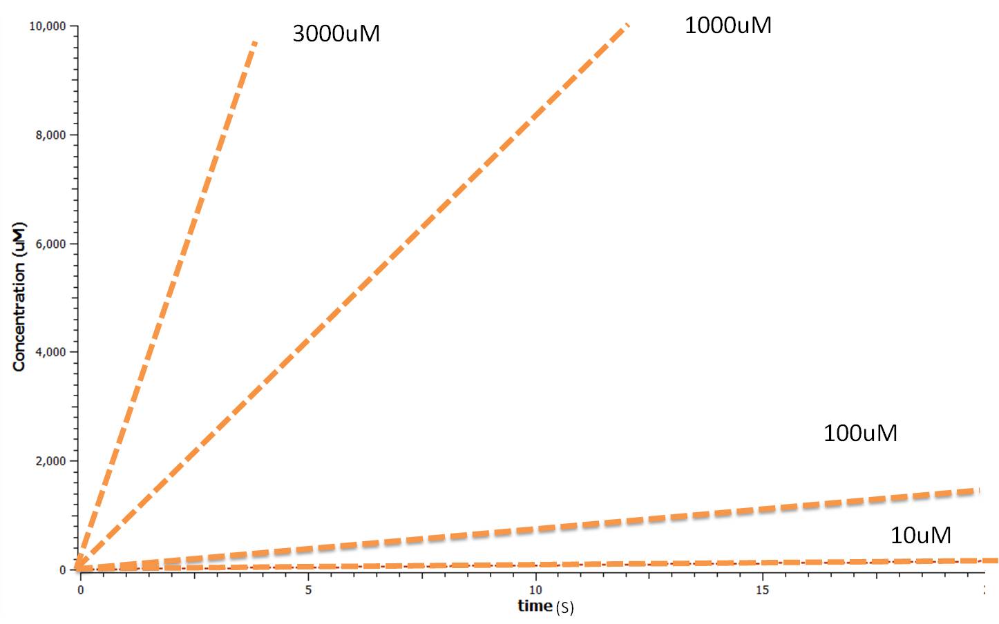
This relatively simple model - as represented in figure 2 - was designed to be the starting point of our kinetic modelling. This uncomplicated system could then be used to obtain an ethylene output. This design comprised only of three enzymes and lacked the transcription and translation stages. The enzymes involved were SAM synthetase, ACC synthase and ACC oxidase - also known as EFE (ethylene forming enzyme). These enzymes were present at fixed concentrations (10, 100, 1000 and 3000 uM) and in a 1:1:1 ratio. Although basic, this model in essence was able to give reasonable output values for ethylene produced. Furthermore with fixed enzyme concentrations the rate at which ethylene is produced depends on the Vmax of the specific enzymes.

This specific rate is defined by the Michaelis-Menton Equation:

         kcat*[substrate]*[enzyme]
Rate =   -------------------------
             km + [substrate]

---

Assumptions for Model 1

- A 1:1:1 steady state of enzymes.

- No product inhibition.

-Substrates (ATP, L-Methionine etc) kept at a constant value due to homeostatic mechanisms in E.coli.

- The best value (km, kcat etc) was always chosen to ensure maximum yield of ethylene.

---

Parameters and Values used

Met concentration - 150 uM

ATP concentration - 9600 uM

O2 concentration - 442 uM

SAMsynth Km(Met)- 92 uM

ACCsynth Km(AdoMet/SAM)- 37 uM

EFE Km(ACC)- 12 uM

SAMsynth turnover rate (kcat)- 1.5 per second

ACCsynth turnover rate (kcat)- 18 per second

EFE turnover rate (kcat) - 5.9 per second

---

Graphs and results

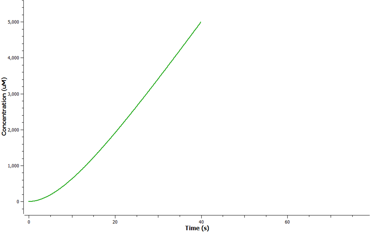
Using Tinkercell a graphical representation of 'Model 1' was generated (Figure 3) using deterministic stimulation. In this figure a graphical representation of the rates - generated internally by Tinkercell's mathematical alogarithms - of ethylene production are shown for each fixed enzyme concentration assumed. As a result not only is production of ethylene shown to be increasing linearly with time, but at a greater rate with increasing concentration of enzyme (SAM synthetase, ACC synthase, EFE) used.

-

Model 2

Model 2 explores the more complicated adaptation of model 1 by incorporating the transcription, translation, and degradation rates of protein and mRNA into the final design. As a result a more realistic model of what would really be happening in the cell leading to ethylene production could be achieved. Of all the sources studied, it was decided that values from the [http://www.ebi.ac.uk/biomodels-main/BIOMD0000000012 Elowitz repressilator model] would be most sensible and relevant to our system. Therefore the degradation, transcription and translation rates were adapted from this model onto ours to factor in fluctuations in concentrations of our three enzymes, as unlike in model 1, enzyme concentration would not realistically be in a 1:1:1 ratio. Therefore using these values, model 2 was able to more realistically follow the metabolic pathway of ethylene production where fluctuations in enzyme concentration were taken into consideration – rather than having them fixed as in model 1.

---

Elowitz Degradation Values

mRNA degradation rate - 0.00577 mRNA per second

Enzyme degradation rate - 0.001155 enzymes per second

R0011 PoPs or transcription rate - 0.5 mRNA per second

Translation rate -0.117 enzymes per second

---

Graphs and results

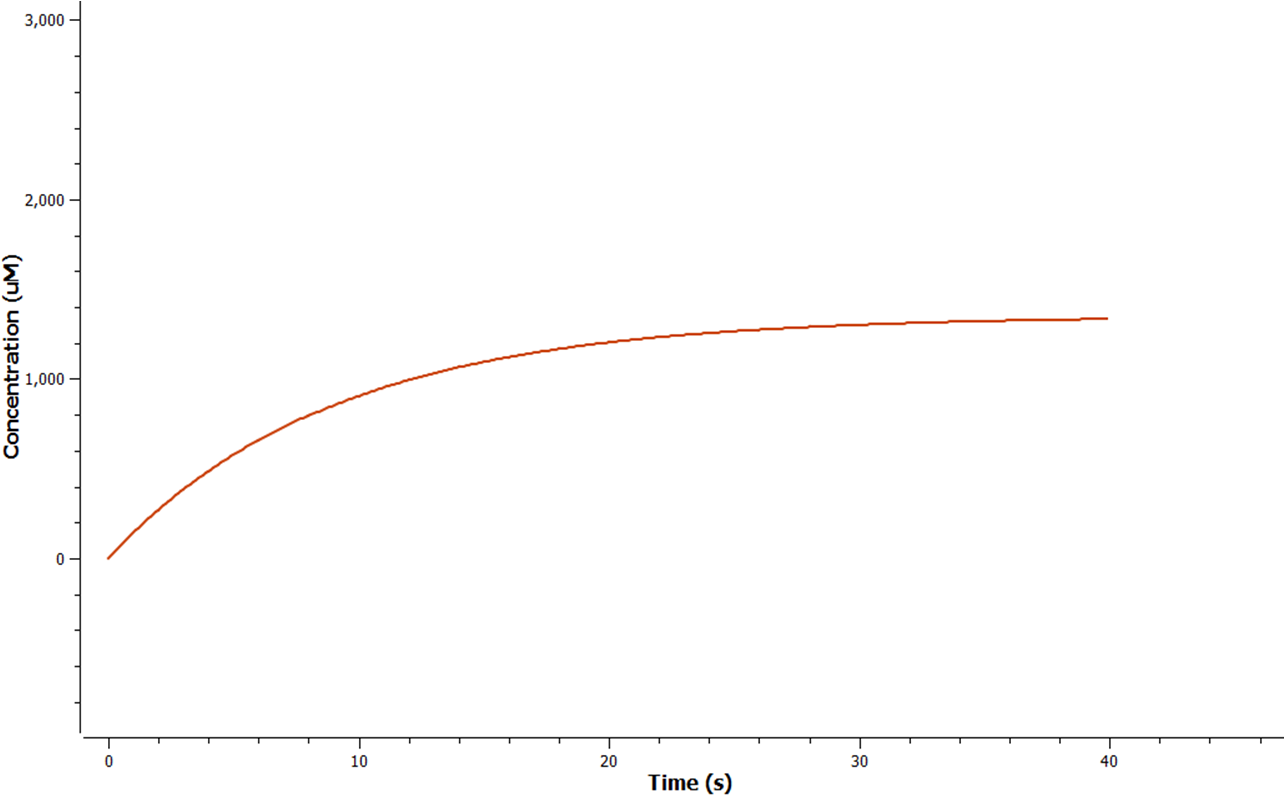
The rate at which mRNA is produced can be seen to start off at a rapid rate. However as time goes on the mRNA can be seen to reach a steady state.

Due to the polycystronic translation of the mRNA all the three enzymes are produced in a 1:1:1 ratio. To begin the enzymes are produced at a realitively fast rate however as time proceeds they fail to reach a steady state. In E.coli it is known that all enzymes eventually reach a steady state otherwise energy and resources would be depleated. Hence this graph suggests plausibility for approximately the first 10 seconds of production; sfter that the data looks unrealistic and implausible in an E.coli cell.

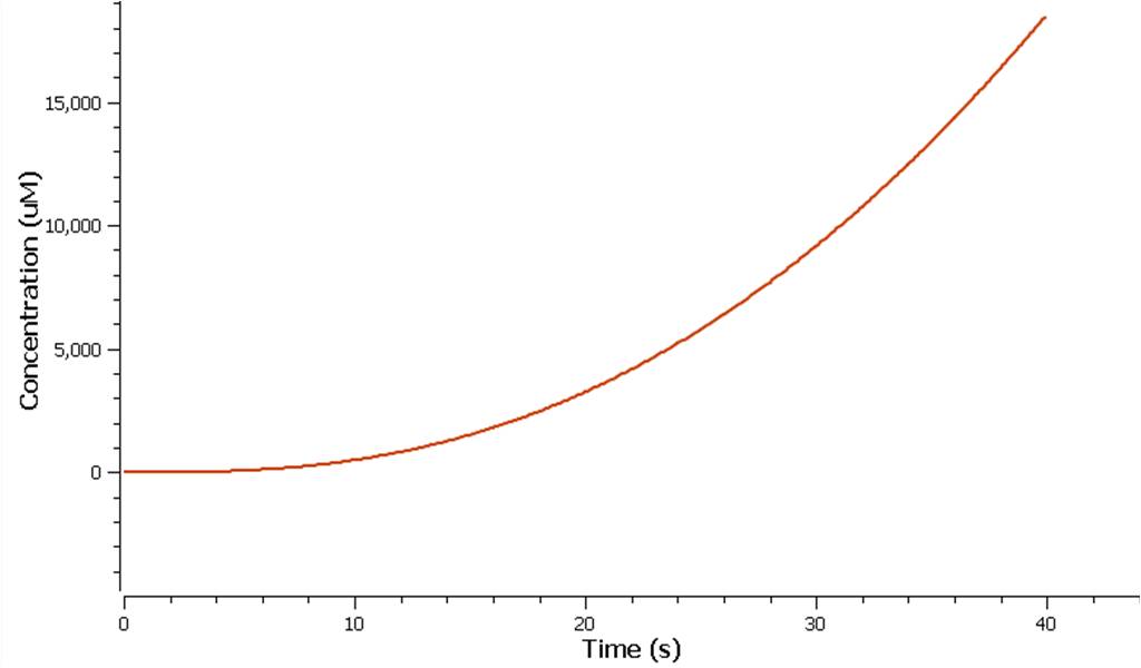
The production of ethylene in this graph looks realitively accurate, however due to the confunding aspects of excess enzyme production, it is unclear if this graph truly represents the total ethylene output. However it can be assumed that the first few seconds accurately portray the ethylene output.