Team:St Andrews/project/modelling/models/RK4
From 2010.igem.org
(→Mathematical basis) |
|||
| Line 38: | Line 38: | ||
| - | [[Image:Picture 4.png]] | + | [[Image:Picture 4.png|600px]] |
| - | + | ||
=References= | =References= | ||
[1] Barker.C.A, "Numerical Methods for Solving Differential Equations,The Runge-Kutta Method, Theoretical Introduction", San Joaquin Delta College, 2009 http://calculuslab.deltacollege.edu/ODE/7-C-3/7-C-3-h.html, [Accessed 13 September 2010] | [1] Barker.C.A, "Numerical Methods for Solving Differential Equations,The Runge-Kutta Method, Theoretical Introduction", San Joaquin Delta College, 2009 http://calculuslab.deltacollege.edu/ODE/7-C-3/7-C-3-h.html, [Accessed 13 September 2010] | ||
Revision as of 11:28, 13 September 2010


Foruth Order Runge-Kutta Method
Introduction
Our method of solving differential equations is based on Fourth Order Runge-Kutta Method. This technique is the most widely used way of numerically solving differential equations and various methods of implementation were looked at. Most of our coding has been based on the work of Aberdeen 2009 iGEM team who used the same method in their modelling. We would like to thank the team for their work and making it available to others like us for future use.
Mathematical basis
While the strict mathematical derivation of the Runge-Kutta method is available( see [http://www.ss.ncu.edu.tw/~lyu/lecture_files_en/lyu_NSSP_Notes/Lyu_NSSP_AppendixC.pdf here for details] ), we omit it here and instead give a brief explanation of the principles behind the technique.
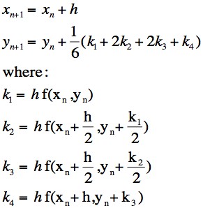
There are several key formulae in the 4th Order Runge-Kutta algorithm, which are:
The iteration of the x-values is done very simply adding a fixed step-size (h) at each iteration, thus resulting in a constant increase in the x-value according to the value of h chosen for a particular purpose.
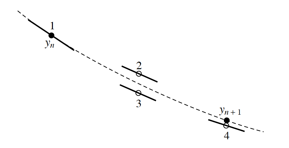
The y-value iteration contains a much more elegant set of relationships. It should be clear to you that the y-iteration formula is in fact a weighted average of the four value k values, k1, k2, k3 and k4. Even at a first glance it should also be apparent that a 'weight' of 2/6 is given to k2 and k3 while a smaller weighting of 1/6 is attributed to k1 and k2. What then do these k-value correspond to geometrically?
Look first at k1. It is equal to the function f(xn,yn) multiplied by the step-size h, which is just the Euler prediction for Δy. It is the vertical distance from the previous point to the next Euler-predicted point.
Then consider k2. It should be noted that the x-value at which the function is being evaluated is halfway across the prediction interval and the y-value consists of the current y-value plus half of the Euler predicted Δy. So then the function is evaluated at a point lying halfway between the current point and the Euler-predicted next point. When we evaluate the function at this point what is produced is an estimate of the slope of the solution curve at this halfway point on curve. Multiplying this result by h gives a prediction of the y-jump made by the solution across the entire interval. However, this prediction is made not on the slope of the solution at the left end of the interval but on the estimated slope halfway to the next Euler-predicted point.
A comparison can be made between k3 and k2, with the only difference in their formulation being the replacement of k1 by k2. Here the function evaluated at this point gives an estimate of the solution slope at the midpoint of the prediction interval but one which is based in the y-jump predicted by k2 rather than the Euler-predicted one. When multiplied by h we get a further estimate of the y-jump made by the solution across the whole interval.
Finally, k4 evaluates the function at the right-hand side of the prediction interval. The y-value at which the function is evaluated, yn+k3 is an estimate of the y-value at the right-hand side based on the estimate of the y-jump made by k3. In its entirey, k4 gives a final estimate of the y-jump made by the solution across the entire width of the prediction interval.
So to provide a summary: each ki yields an estimate of the y-jump made by the solution across the entire width of the prediction interval h, with each using the previous ki to make its estimate. The Runge-Kutta formula can be viewed as the y-value of the current point plus a weighted average of four different predictions for the slope.
References
[1] Barker.C.A, "Numerical Methods for Solving Differential Equations,The Runge-Kutta Method, Theoretical Introduction", San Joaquin Delta College, 2009 http://calculuslab.deltacollege.edu/ODE/7-C-3/7-C-3-h.html, [Accessed 13 September 2010]
 "
"

