Team:BCCS-Bristol/Modelling/GRN/Derivation
From 2010.igem.org
m |
|||
| (3 intermediate revisions not shown) | |||
| Line 2: | Line 2: | ||
=Derivation= | =Derivation= | ||
| - | |||
| - | |||
==GRN Model== | ==GRN Model== | ||
| + | {{:Team:BCCS-Bristol/newtoc}} | ||
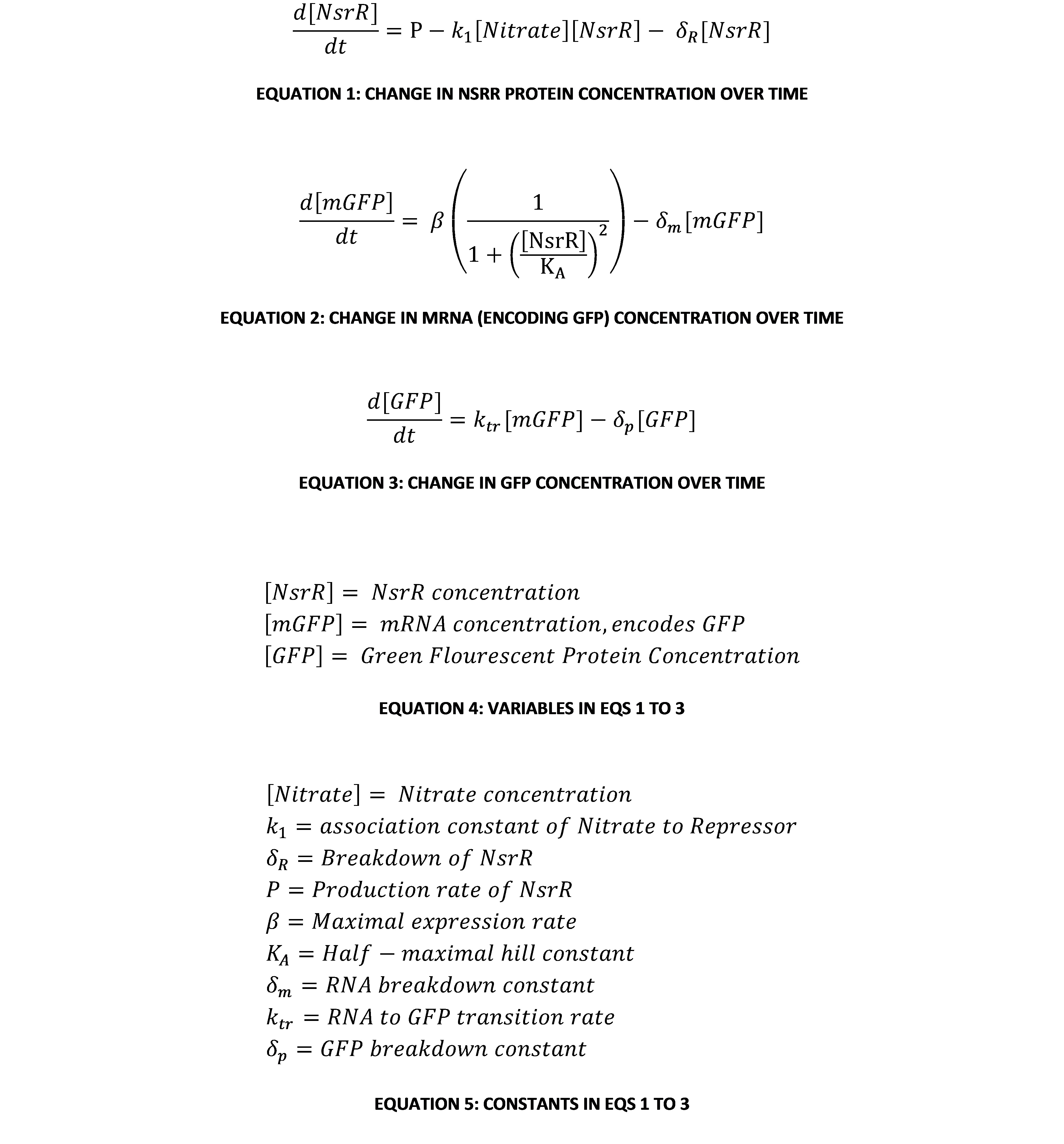
A Gene Regulatory Network (GRN) model is an established way of representing the biochemical reactions within a bacterial cell [1]. Representing a network of interacting components using differential equations can be very useful, mainly because one can make analytical and qualitative assessments of a system’s behaviour with very limited information on parameters. This GRN represents a protein called NsrR that represses the production of mRNA encoding GFP, and so indirectly repressing the production of GFP. NsrR can bind to breakdown products of nitrates, effectively destroying its ability to repress the system. Since nitrates in soil have a long time to break down before agrEcoli is used, we can model the quantity of nitrate breakdown products as being indicative of the quantity of nitrates in the soil. As such, our GRN model has nitrates binding directly to NsrR; while this isn't strictly true, it is a justified simplification. | A Gene Regulatory Network (GRN) model is an established way of representing the biochemical reactions within a bacterial cell [1]. Representing a network of interacting components using differential equations can be very useful, mainly because one can make analytical and qualitative assessments of a system’s behaviour with very limited information on parameters. This GRN represents a protein called NsrR that represses the production of mRNA encoding GFP, and so indirectly repressing the production of GFP. NsrR can bind to breakdown products of nitrates, effectively destroying its ability to repress the system. Since nitrates in soil have a long time to break down before agrEcoli is used, we can model the quantity of nitrate breakdown products as being indicative of the quantity of nitrates in the soil. As such, our GRN model has nitrates binding directly to NsrR; while this isn't strictly true, it is a justified simplification. | ||
[[Image:GRN.jpg|frameless|center|upright=4|agrEcoli Gene Regulatory Network Equations]] | [[Image:GRN.jpg|frameless|center|upright=4|agrEcoli Gene Regulatory Network Equations]] | ||
| + | |||
==Analysis== | ==Analysis== | ||
| Line 28: | Line 28: | ||
[[Image:BCCS_GRN_EQ_9.jpg|frameless|center|upright=4|BCCS-Bristol GRN equation 9]] | [[Image:BCCS_GRN_EQ_9.jpg|frameless|center|upright=4|BCCS-Bristol GRN equation 9]] | ||
| + | |||
==Fixed Point Solution== | ==Fixed Point Solution== | ||
| Line 34: | Line 35: | ||
[[Image:BCCS_GRN_EQ_10.jpg|frameless|center|upright=4|BCCS-Bristol GRN equation 10]] | [[Image:BCCS_GRN_EQ_10.jpg|frameless|center|upright=4|BCCS-Bristol GRN equation 10]] | ||
| + | |||
==References== | ==References== | ||
Latest revision as of 18:36, 27 October 2010
iGEM 2010
Derivation
GRN Model
A Gene Regulatory Network (GRN) model is an established way of representing the biochemical reactions within a bacterial cell [1]. Representing a network of interacting components using differential equations can be very useful, mainly because one can make analytical and qualitative assessments of a system’s behaviour with very limited information on parameters. This GRN represents a protein called NsrR that represses the production of mRNA encoding GFP, and so indirectly repressing the production of GFP. NsrR can bind to breakdown products of nitrates, effectively destroying its ability to repress the system. Since nitrates in soil have a long time to break down before agrEcoli is used, we can model the quantity of nitrate breakdown products as being indicative of the quantity of nitrates in the soil. As such, our GRN model has nitrates binding directly to NsrR; while this isn't strictly true, it is a justified simplification.
Analysis
The most interesting relationship in this system of equations is the relationship between the concentration of NsrR repressor protein and the concentration of GFP in the system. A useful way of visualising and analysing the system’s dynamics is using a phase plane portrait in 2 dimensions. However, this means eliminating one of the variables. This can be done by making an equilibrium assumption about the amount of mRNA encoding GFP (mGFP for short). To do this, we set Equation 2 equal to 0. Rearranging in terms of [mGFP], this gives:
This can be substituted into Equation 3 to give an expression of [GFP] in terms of only itself and [NsrR]. This is now a system of 2 variables, so with a little further manipulation it can be put into a phase-plane portrait. The system of 2 linear ODEs is:
By taking the Jacobian http://mathworld.wolfram.com/Jacobian.html 2 of these equations, we can classify the dynamics of the system. The eigenvalues of the Jacobian matrix, M, determine the system’s dynamic states.
The eigenvalues of this matrix are:
Fixed Point Solution
Since all the constants in this system of equations are constrained to be real semi-positive numbers (i.e. ≥0), both eigenvalues are always real and negative. This means that the only fixed point on the phase-plane will be a stable node (possibly degenerate or improper). Further, it is impossible for either eigenvalue to be 0 as both breakdown constants of GFP and NsrR are known to be explicitly positive (i.e. >0). Thus it is clear that the system always converges to a single equilibrium point. By finding the nullclines of the equation and working out where they meet, the fixed point can be found:
References
| [1] | Alon, Uri An Introduction to Systems Biology: Design Principles of Biological Circuits. London : Chapman & Hall, 2006. |
| http://mathworld.wolfram.com/Jacobian.html 2 | Wolfram Jacobian |
 "
"


