Team:BCCS-Bristol/Modelling/BSIM/Modelling Environmental Interactions
From 2010.igem.org
(New page: {{:Team:BCCS-Bristol/Header}} =Modelling Environmental Interactions= ==Introduction== BSim carries out its simulations in a three dimensional space, this is necessary for many simulatio...) |
|||
| Line 5: | Line 5: | ||
==Introduction== | ==Introduction== | ||
| - | BSim carries out its simulations in a three dimensional space | + | {{:Team:BCCS-Bristol/newtoc}} |
| + | |||
| + | BSim carries out its simulations in a three dimensional space. This is necessary for many simulations | ||
involving populations of bacteria and modelling their interactions. In figure 1, for example, you | involving populations of bacteria and modelling their interactions. In figure 1, for example, you | ||
can see an example of bacteria emitting and merging with vesicles in three dimensions. They are | can see an example of bacteria emitting and merging with vesicles in three dimensions. They are | ||
| - | modelled as being in water, with | + | modelled as being in water, with periodic boundary conditions (meaning that if you go out of |
the top of the box you re-appear at the bottom). This creates a continuous domain, which is fine | the top of the box you re-appear at the bottom). This creates a continuous domain, which is fine | ||
for modelling the conditions inside a test tube where the environment is large enough compared to | for modelling the conditions inside a test tube where the environment is large enough compared to | ||
| - | the items being modelled that it is | + | the items being modelled that it is effectively infinite. |
Some of the modelling questions that we want to answer in this project pertain to environments | Some of the modelling questions that we want to answer in this project pertain to environments | ||
| - | that are of the same scale as the bacteria. One important question is how E. coli move inside the | + | that are of the same scale as the bacteria. One important question is how <i>E. coli</i> move inside the |
| - | micro-structure of the gellan beads gel matrix (figure 2). This is important as it will determine how much of the E. coli escapes the bead environment over time. Another question that could be answered via accurate | + | micro-structure of the gellan beads' gel matrix (figure 2). This is important as it will determine how much of the <i>E. coli</i> escapes the bead environment over time. Another question that could be answered via accurate |
| - | modelling of surfaces in BSim would be how exactly nitrate | + | modelling of surfaces in BSim would be how exactly nitrate diffuses from the soil contact area of |
the bead and into the micro-structure of the gellan bead. This would provide an insight into how | the bead and into the micro-structure of the gellan bead. This would provide an insight into how | ||
homogeneous the nitrate concentrations inside the bead are. | homogeneous the nitrate concentrations inside the bead are. | ||
| + | <gallery widths=200px> | ||
| + | Image:BsimVesicle.png|Figure 1 | ||
| + | Image:Depth0.png|Figure 2 | ||
| + | </gallery> | ||
| - | + | <html> | |
| - | + | <center> | |
| - | + | <object width="425" height="344"><param name="movie" value="http://www.youtube.com/v/joMxPbb09Ds?fs=1&hl=en_GB"></param><param name="allowFullScreen" value="true"></param><param name="allowscriptaccess" value="always"></param><embed src="http://www.youtube.com/v/joMxPbb09Ds?fs=1&hl=en_GB" type="application/x-shockwave-flash" allowscriptaccess="always" allowfullscreen="true" width="425" height="344"></embed></object> | |
| - | + | ||
| - | + | ||
| - | < | + | |
| - | < | + | |
| - | + | ||
| - | + | ||
| - | + | ||
| - | + | ||
| - | + | ||
| - | + | ||
| - | + | ||
| - | + | ||
| - | + | ||
| - | + | ||
| - | + | ||
| - | + | <object width="425" height="344"><param name="movie" value="http://www.youtube.com/v/7ourSYT8Oug?fs=1&hl=en_GB"></param><param name="allowFullScreen" value="true"></param><param name="allowscriptaccess" value="always"></param><embed src="http://www.youtube.com/v/7ourSYT8Oug?fs=1&hl=en_GB" type="application/x-shockwave-flash" allowscriptaccess="always" allowfullscreen="true" width="425" height="344"></embed></object> | |
| + | </center> | ||
| + | </html> | ||
=Implementation= | =Implementation= | ||
| Line 57: | Line 50: | ||
==Collisions== | ==Collisions== | ||
| + | |||
| + | [[Image:Teapot_Mesh.png|200px|thumb|left|fig 1]] | ||
As well as implementing meshes into BSim, we also added routines for computing collision events. This allows the user to detect when any object comes into contact with a mesh boundary and to respond as required. Although the default behaviour of BSim is to use the mesh as a boundary to restrict bacterial movement, it is trivial to add other responses. Possible complex responses include detecting the collision of chemicals, for example proteins, with a cell surface represented by a mesh boundary, or extending BSim to include biofilms. | As well as implementing meshes into BSim, we also added routines for computing collision events. This allows the user to detect when any object comes into contact with a mesh boundary and to respond as required. Although the default behaviour of BSim is to use the mesh as a boundary to restrict bacterial movement, it is trivial to add other responses. Possible complex responses include detecting the collision of chemicals, for example proteins, with a cell surface represented by a mesh boundary, or extending BSim to include biofilms. | ||
| - | + | <br/><br/><br/><br/> | |
==Computing Diffusion== | ==Computing Diffusion== | ||
| - | The diffusion of chemicals across the chemical | + | The diffusion of chemicals across the chemical field must be also computed. This involves |
| - | solving a | + | solving a differential equation across an arbitrarily shaped 3D space. There are two broad classes |
| - | of methods that are used to do this, | + | of methods that are used to do this, finite element methods and finite difference methods. |
| - | A | + | A finite element approach would use the mesh as a basis to generate a series of discrete units |
| - | across which to calculate a | + | across which to calculate a discretised approximation system of ordinary differential equations. This |
| - | is | + | is difficult to do reliably with arbitrary shapes. There exist several different algorithms that work |
| - | well with | + | well with different types of spaces (smooth, jagged, convex, concave) but it is difficult to implement |
| - | a | + | a finite element method that works reliably in an arbitrary geometry without numerical instability. |
| - | An example of a tessellation of triangles used to compute a | + | An example of a tessellation of triangles used to compute a finite element method approach can be |
| - | seen in | + | seen in fig. 2(a). An accurate finite element model would converge to the analytical solution as the |
| - | mesh became | + | mesh became finer and finer, unfortunately this is difficult to do in generality, such a model which |
would be necessary for a robust addition to this modelling framework. | would be necessary for a robust addition to this modelling framework. | ||
| - | A | + | A finite difference method discretises and computes a differential equation over a regular lattice, |
| - | e.g. | + | e.g. fig. 2(b) This means that it is much more numerically stable than the finite element method. |
| - | The trade- | + | The trade-off is that you have to partition the space along the lines of this regular grid. Which is not |
a very accurate representation of curves unless the resolution of the lattice is very high compared | a very accurate representation of curves unless the resolution of the lattice is very high compared | ||
to the resolution of the curved object that you wanted to represent. | to the resolution of the curved object that you wanted to represent. | ||
| - | + | <gallery widths=200px> | |
| - | + | Image:FEM.png|fig 2a | |
| - | + | Image:FDM.png|fig 2b | |
| - | + | </gallery> | |
The solution that we decided to use to implement the chemical field processing is an ' [[Team:BCCS-Bristol/Modelling/BSIM/Geometric_Modelling/Octrees|octree]]' structure. This is a hybrid between the two methods, though is more closely related to the finite | The solution that we decided to use to implement the chemical field processing is an ' [[Team:BCCS-Bristol/Modelling/BSIM/Geometric_Modelling/Octrees|octree]]' structure. This is a hybrid between the two methods, though is more closely related to the finite | ||
| Line 97: | Line 92: | ||
with respect to its memory requirements because it only divides itself into a high resolution where | with respect to its memory requirements because it only divides itself into a high resolution where | ||
necessary. | necessary. | ||
| - | |||
| - | |||
| - | |||
=Octrees= | =Octrees= | ||
==Overview== | ==Overview== | ||
| + | |||
| + | [[Image:OctreeSchem.png|250px|thumbnail|right|Fig. 1. Schematic illustration of how an octree subdividies in space (left) and how this is represented as a node and leaf data structure (right). In this example the highest resolution node | ||
| + | is of depth 3.]] | ||
| + | |||
The octree is a tree type data structure. This a hierarchical data structure comprised of nested | The octree is a tree type data structure. This a hierarchical data structure comprised of nested | ||
nodes. Each node has one parent and either eight or zero children. Nodes with zero children are | nodes. Each node has one parent and either eight or zero children. Nodes with zero children are | ||
| Line 110: | Line 106: | ||
be represented by a tree data structure. | be represented by a tree data structure. | ||
| - | + | <br/><br/><br/><br/><br/><br/><br/><br/><br/><br/><br/><br/> | |
| - | + | ||
| - | + | ||
==Methods== | ==Methods== | ||
| Line 141: | Line 135: | ||
==Splitting the Octree== | ==Splitting the Octree== | ||
| + | |||
| + | [[Image:Quadtree.png|250px|thumbnail|right|Fig. 2. An example of quadtree partitioning, as the maximum depth increases, the partition more closely approximates the curve]] | ||
| + | |||
The octree data structure is used for holding and computing the chemical field because it is able | The octree data structure is used for holding and computing the chemical field because it is able | ||
to approximately represent fields of arbitrary shapes. This is done by splitting an octree from a | to approximately represent fields of arbitrary shapes. This is done by splitting an octree from a | ||
parent node around a mesh shape. It is easier to explain in terms of the two dimensional quadtree, | parent node around a mesh shape. It is easier to explain in terms of the two dimensional quadtree, | ||
| - | the principle is exactly the same for an octree, an example is shown in fig. 2. | + | the principle is exactly the same for an octree, an example is shown in fig. 2. |
| - | + | ||
This example has a maximum depth of three, the example of an octree partition in fig. 2 has a depth of 5. The | This example has a maximum depth of three, the example of an octree partition in fig. 2 has a depth of 5. The | ||
| Line 154: | Line 150: | ||
traverse function above to access each octree node from the bottom to the top. The following | traverse function above to access each octree node from the bottom to the top. The following | ||
function would be in place of the ‘VISIT’ command: | function would be in place of the ‘VISIT’ command: | ||
| + | |||
| + | <br/><br/><br/> | ||
<pre> | <pre> | ||
| Line 176: | Line 174: | ||
<center><html><object width="425" height="344"><param name="movie" value="http://www.youtube.com/v/Uoh1mCADghI?fs=1&hl=en_US&rel=0&hd=1"></param><param name="allowFullScreen" value="true"></param><param name="allowscriptaccess" value="always"></param><embed src="http://www.youtube.com/v/Uoh1mCADghI?fs=1&hl=en_US&rel=0&hd=1" type="application/x-shockwave-flash" allowscriptaccess="always" allowfullscreen="true" width="425" height="344"></embed></object></html></center> | <center><html><object width="425" height="344"><param name="movie" value="http://www.youtube.com/v/Uoh1mCADghI?fs=1&hl=en_US&rel=0&hd=1"></param><param name="allowFullScreen" value="true"></param><param name="allowscriptaccess" value="always"></param><embed src="http://www.youtube.com/v/Uoh1mCADghI?fs=1&hl=en_US&rel=0&hd=1" type="application/x-shockwave-flash" allowscriptaccess="always" allowfullscreen="true" width="425" height="344"></embed></object></html></center> | ||
| - | |||
| - | |||
| - | |||
| - | |||
| - | |||
| - | |||
| - | |||
| - | |||
| - | |||
| - | |||
| - | |||
Revision as of 18:12, 27 October 2010
iGEM 2010
Modelling Environmental Interactions
Introduction
Contents |
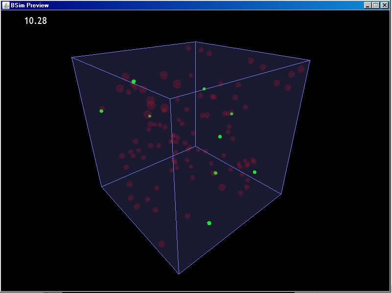
BSim carries out its simulations in a three dimensional space. This is necessary for many simulations involving populations of bacteria and modelling their interactions. In figure 1, for example, you can see an example of bacteria emitting and merging with vesicles in three dimensions. They are modelled as being in water, with periodic boundary conditions (meaning that if you go out of the top of the box you re-appear at the bottom). This creates a continuous domain, which is fine for modelling the conditions inside a test tube where the environment is large enough compared to the items being modelled that it is effectively infinite.
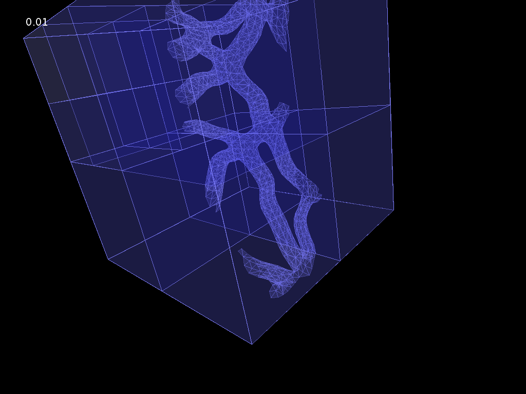
Some of the modelling questions that we want to answer in this project pertain to environments that are of the same scale as the bacteria. One important question is how E. coli move inside the micro-structure of the gellan beads' gel matrix (figure 2). This is important as it will determine how much of the E. coli escapes the bead environment over time. Another question that could be answered via accurate modelling of surfaces in BSim would be how exactly nitrate diffuses from the soil contact area of the bead and into the micro-structure of the gellan bead. This would provide an insight into how homogeneous the nitrate concentrations inside the bead are.
Implementation
Overview
There are two computational structures that need to take account of complex three dimensional structures if these features are to be implemented. One is the ability to represent a 3D shape inside the BSim environment, for example to provide a boundary, the other is the ability to represent a chemical field defined by such a 3D shape.
Representing 3D Shapes
In the early design phase of AgrEcoli, it quickly became evident that we would need to simulate some form of interaction between a bacterial population and its environment. Common analytical shapes (those that can be defined directly via a set of equations, for example a sphere) are somewhat limited when it comes to representing real-world objects. Fortunately there are a number of methods for specifying an arbitrary boundary in three dimensional space, such as through a set of parametric curves or via constructive solid geometry (often this involves combining a set of analytical shapes). However, the most common method throughout the field of computational geometry is to use a polyhedral mesh.
A polyhedral mesh can represent almost any three dimensional structure to an arbitrary degree of precision, so it was this type of 3D structure that we decided to use to represent boundaries. BSim currently supports arbitrary triangle-based meshes, which may contain both convex and concave regions as well as holes. Triangle meshes are the most common type of mesh output from computational geometry algorithms and from 3D modelling software, and are the simplest and most robust type of mesh one can use; almost any meshes of greater complexity can be simplified to a triangle mesh. BSim implements triangle meshes using a face-vertex representation internally. It currently supports direct import of .OBJ files, one of the most common file formats used for exchange of 3D mesh information, and standardised across the industry.
Collisions
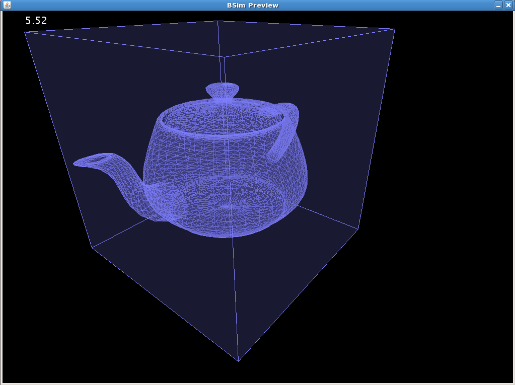
As well as implementing meshes into BSim, we also added routines for computing collision events. This allows the user to detect when any object comes into contact with a mesh boundary and to respond as required. Although the default behaviour of BSim is to use the mesh as a boundary to restrict bacterial movement, it is trivial to add other responses. Possible complex responses include detecting the collision of chemicals, for example proteins, with a cell surface represented by a mesh boundary, or extending BSim to include biofilms.
Computing Diffusion
The diffusion of chemicals across the chemical field must be also computed. This involves solving a differential equation across an arbitrarily shaped 3D space. There are two broad classes of methods that are used to do this, finite element methods and finite difference methods.
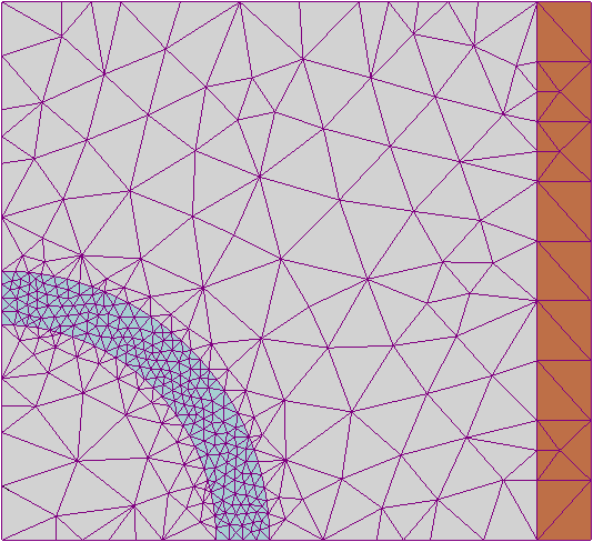
A finite element approach would use the mesh as a basis to generate a series of discrete units across which to calculate a discretised approximation system of ordinary differential equations. This is difficult to do reliably with arbitrary shapes. There exist several different algorithms that work well with different types of spaces (smooth, jagged, convex, concave) but it is difficult to implement a finite element method that works reliably in an arbitrary geometry without numerical instability. An example of a tessellation of triangles used to compute a finite element method approach can be seen in fig. 2(a). An accurate finite element model would converge to the analytical solution as the mesh became finer and finer, unfortunately this is difficult to do in generality, such a model which would be necessary for a robust addition to this modelling framework.
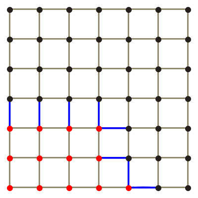
A finite difference method discretises and computes a differential equation over a regular lattice, e.g. fig. 2(b) This means that it is much more numerically stable than the finite element method. The trade-off is that you have to partition the space along the lines of this regular grid. Which is not a very accurate representation of curves unless the resolution of the lattice is very high compared to the resolution of the curved object that you wanted to represent.
The solution that we decided to use to implement the chemical field processing is an ' octree' structure. This is a hybrid between the two methods, though is more closely related to the finite difference method. This uses a regular lattice of cubes, but changes the resolution of the lattice as it is partitioned by a mesh surface. This technique is visualized in fig. 10, note how the lattice resolution increases around the sphere mesh, this allows for a more accurate division of the lattice into a sphere shape. An octree structure will never be able to perfectly duplicate the shape of the mesh that it is cast from, but the maximum resolution can be far higher than a regular lattice with respect to its memory requirements because it only divides itself into a high resolution where necessary.
Octrees
Overview
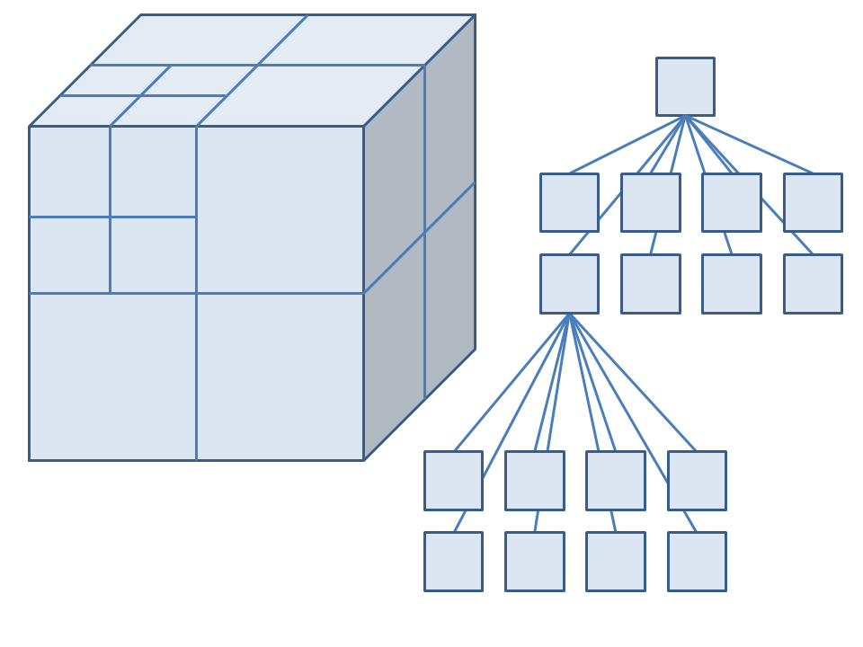
The octree is a tree type data structure. This a hierarchical data structure comprised of nested nodes. Each node has one parent and either eight or zero children. Nodes with zero children are called leaves. A node's children subdivide the volume of their parent into eight smaller volumes. Figure 1 shows how an octree partitions space into smaller and smaller volumes and how this can be represented by a tree data structure.
Methods
Each node stores the quantity of chemical and the diffusivity constant for its field. Nodes know what depth they are inside the octree structure and which nodes are their neighbours. This is re-computed each time a node is split it is necessary to know who your neighbors are in order to compute the diffusion of chemicals through the field from one node to those spatially adjacent (i.e. not necessarily nodes of the same parent).
To be able to perform operations across an octree data structure it is necessary to use a traversal algorithm. This is an algorithm that visits each node. There are many different ways of doing this, the method used in BSim is the ‘full post-order’ traverse. This visits each node from deepest depth first, then the second deepest etcetera until it reaches the parent node.
PostOrderTraverse(Node)

{
    IF(Node != leaf){
        FOR(i=0:8){
        PostOrderTraverse(Node.subNodes[i])}
        VISIT(Node)
   }

}
Splitting the Octree
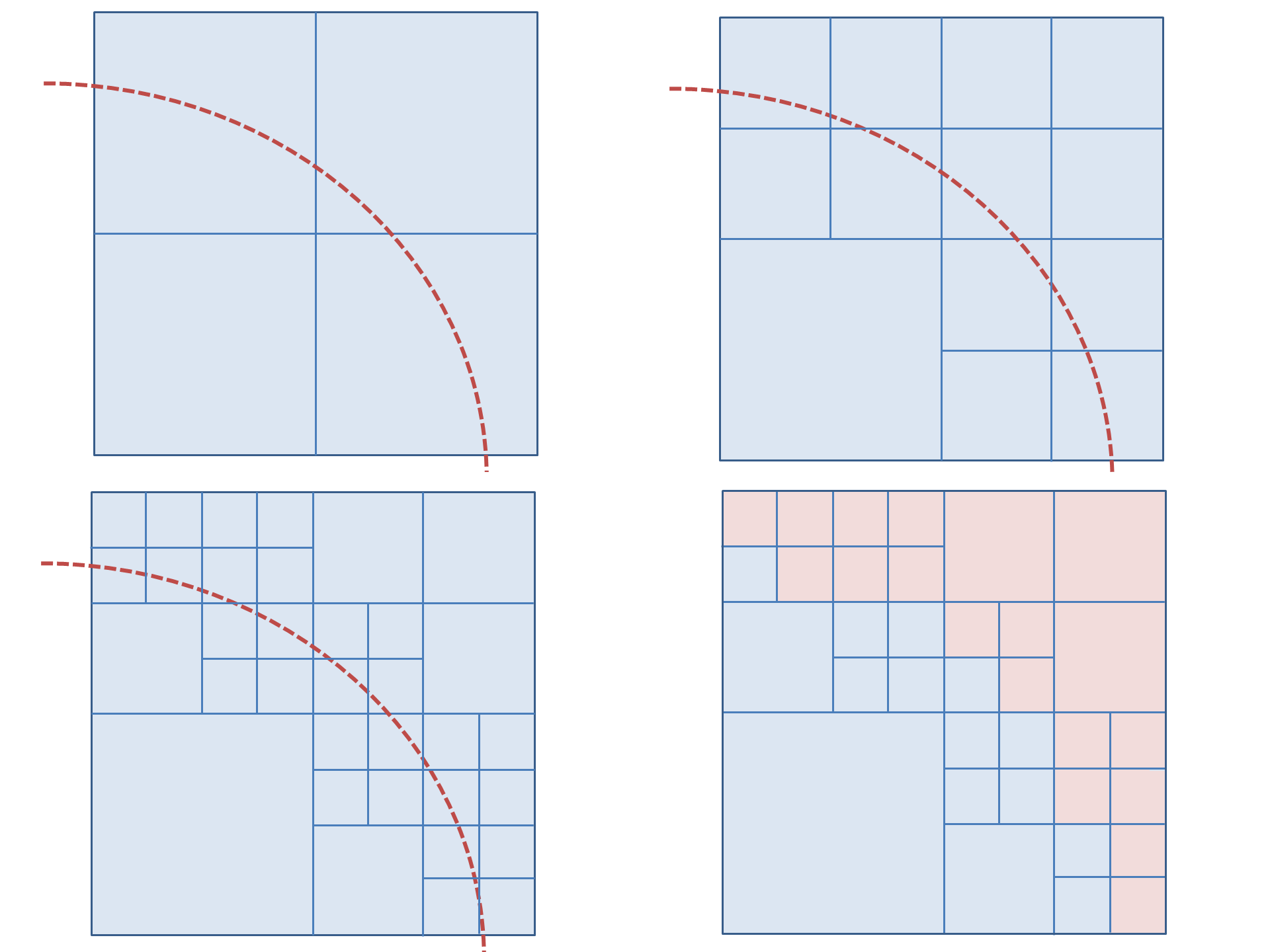
The octree data structure is used for holding and computing the chemical field because it is able to approximately represent fields of arbitrary shapes. This is done by splitting an octree from a parent node around a mesh shape. It is easier to explain in terms of the two dimensional quadtree, the principle is exactly the same for an octree, an example is shown in fig. 2.
This example has a maximum depth of three, the example of an octree partition in fig. 2 has a depth of 5. The maximum resolution increases exponentially with depth, a depth of 7 appears to be adequate for reasonably complex shapes, e.g. the mesh of a gel strand.
The algorithm for splitting the octree around a mesh is relatively simple. It uses the post order traverse function above to access each octree node from the bottom to the top. The following function would be in place of the ‘VISIT’ command:
FOR each Edge of Mesh{
   FOR each Edge of Node{
     IF(Node Edge is crossed by a Mesh Edge)
       Divide Node into SubNodes
     ELSE
       Check next Mesh Edge
   }
}
It is relatively inefficient, each edge of the octree is tested against each edge of the mesh. It could be optimised to try and exclude mesh edges that are extremely unlikely to cross the node edge. It would also be prudent to exclude mesh edges that are too far away from the node to intersect it, as this algorithm would require only addition and subtraction, whereas the collision detection algorithm operates with vector products.
An example of how an octree is split around a mesh in BSim can be seen in the video below. Here you can see how the octree structure looks at each stage of its generation. The maximum resolution increases from 1 at the start, to 8 in the final frame.
 "
"
