|
|
| Line 61: |
Line 61: |
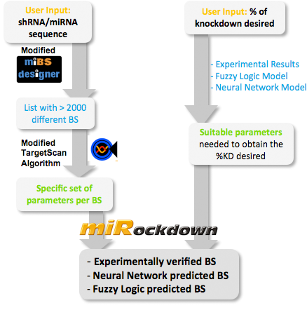
| | miBS designer generates the primer needed to integrate the binding site desired, into a plasmid, alongside with the primer for the complementary strand. It will also produce specific names for the two primers. | | miBS designer generates the primer needed to integrate the binding site desired, into a plasmid, alongside with the primer for the complementary strand. It will also produce specific names for the two primers. |
| | | | |
| - | ==Neural Network Model==
| |
| - | ===Neural Network theory===
| |
| - | Artificial Neural Network usually called (NN), is a computational model that is inspired by the biological nervous system. The network is composed of simple elements called artificial neurons that are interconnected and operate in parallel. In most cases the NN is an adaptive system that can change its structure depending on the internal or(and?) external information that flows into the network during the learning process. The NN can be trained to perform a particular function by adjusting the values of the connection, called weights, between the artificial neurons. Neural Networks have been employed to perform complex functions in various fields, including pattern recognition, identification, classification, speech, vision, and control systems.
| |
| | | | |
| - | During the learning process, difference between the desired output (target) and the network output is minimised. This difference is usually called cost; the cost function is the measure of how far is the network output from the desired value. A common cost function is the mean-squared error and there are several algorithms that can be used to minimise this function. The following figure displays such a loop.
| |
| - | [[Image:network.gif|400px|center]]
| |
| - |
| |
| - | Figure 2: Training of a Neural Network.
| |
| - |
| |
| - | ===Model description===
| |
| - |
| |
| - | ====Input/target pairs====
| |
| - | The NN model has been created with the MATLAB NN-toolbox. The input/target pairs used to train the network comprise experimental and literature data (Bartel et al. 2007). The experimental data were obtained by measuring via luciferase assay the strength of knockdown due to the interaction between the shRNA and the binding site situated on the 3’UTR of luciferase gene. Nearly 30 different rational designed binding sites were tested and the respective knockdown strength calculated with the following formula->(formula anyone???).<br>
| |
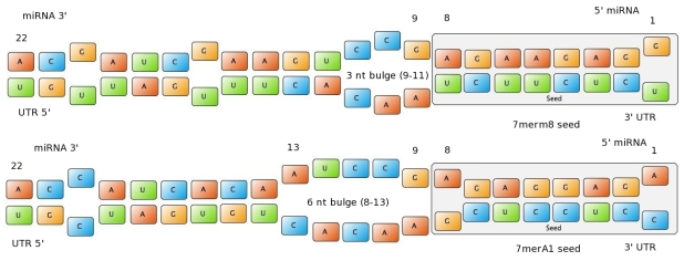
| - | Each input was represented by a four elements vector. Each element corresponded to a score value related to a specific feature of the binding site. The four features used to describe the binding site were: seed type, the 3’pairing contribution the AU-content and the number of binding site. The input/target pair represented the relationship between a particular binding site and the related percentage of knockdown.
| |
| - | The NN was trained with a pool of 46 data. Afterwards it was used to predict percentages of knockdown given certain inputs. The predictions were then validated experimentally.
| |
| - |
| |
| - | ====Characteristic of the Network====
| |
| - |
| |
| - | The neural network comprised two layers (multilayer feedforward Network). The first layer is connected with the input network and it comprised 15 artificial neurons. The second layer is connected to the first one and it produced the output. For the first and the second layer a sigmoid activation function and a linear activation function were used respectively. The algorithm used for minimizing the cost function (sum squared error) was Bayesian regularization. This Bayesian regularization takes place within the Levenberg-Marquardt algorithm. The algorithm updates the weight and bias values according to Levenberg-Marquardt optimization and overcomes the problem in interpolating noisy data, (MacKay 1992) by applying a Bayesian framework to the NN learning problem.<br>
| |
| - | <br>
| |
| - | [[Image:view net.png|center]]<br>
| |
| - | <br>
| |
| - | Figure 3: schematic illustration of the network components. Hidden represent the first layer and it comprised 15 artificial neurons, while output is the second and last layer producing the output. The symbol “w” was the representation of the weights and “b” of the biases.
| |
| - |
| |
| - | ===Results===
| |
| - | ====Training the Neural Network====
| |
| - | The Network was trained with 46 samples. The regression line showing the correlation between the NN outputs and the targets was R=0.9864. <br>
| |
| - | <br>
| |
| - | [[Image:regression.png|300px]] <br>
| |
| - | <br>
| |
| - | Figure 4: Regression line showing the correlation between the NN output and the respective target value.
| |
| - |
| |
| - | <html>
| |
| - | <div class="backtop">
| |
| - | <a href="#top">↑</a>
| |
| - | </div>
| |
| - | </html>
| |
| - | ====Simulation and experimental verification====
| |
| | | | |
| | ==Fuzzy Inference Model== | | ==Fuzzy Inference Model== |

 "
"
