Team:Imperial College London/Modelling/Output/Results and Conclusion
From 2010.igem.org
m |
m |
||
| Line 255: | Line 255: | ||
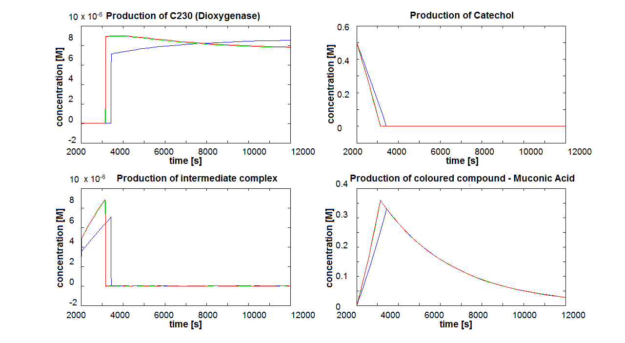
#In case of cells being modelled as alive, the difference between the 2-step amplified and the 1-step amplified model is smaller than it is in case of cell death. | #In case of cells being modelled as alive, the difference between the 2-step amplified and the 1-step amplified model is smaller than it is in case of cell death. | ||
| - | Since it appears that the time of cell death is important, we decided to discuss this issue with | + | Since it appears that the time of cell death is important, we decided to discuss this issue with our team members. Referring to this paper <html><a href="http://www.sciencedirect.com/science?_ob=MImg&_imagekey=B6V78-4XXNV4Y-4-7&_cdi=5836&_user=217827&_pii=S0048969709011668&_orig=search&_coverDate=02%2F01%2F2010&_sk=995919994&view=c&wchp=dGLbVzz-zSkzk&_valck=1&md5=f8dca6227c29db659ddbeb588ad115e7&ie=/sdarticle.pdf">[1]</a></html> we decided that cell death induced by catechool is a very slow process (we estimate that it will take a few hours) in comparison to the time scale that we are interested in (several seconds to minutes). Hence, our final conclusions will be on the model neglecting cell death. |
| - | + | <div ALIGN=Center> | |
| - | + | ||
| - | + | ||
{| style="width:430px;background:#e7e7e7;text-align:center;font-family: helvetica, arial, sans-serif;color:#555555;margin- top:5px;padding: 1px;" cellspacing="5"; | {| style="width:430px;background:#e7e7e7;text-align:center;font-family: helvetica, arial, sans-serif;color:#555555;margin- top:5px;padding: 1px;" cellspacing="5"; | ||
|- | |- | ||
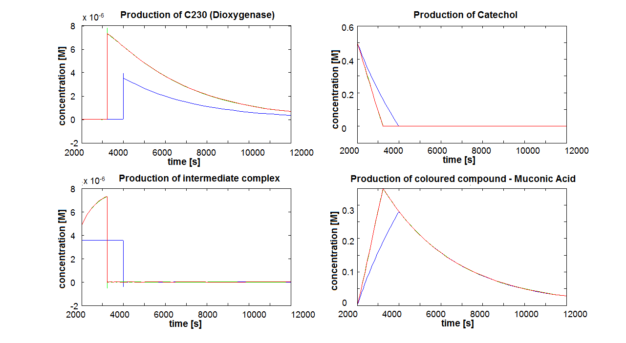
| - | |[[Image:IC_alive_cells.png| | + | |[[Image:IC_alive_cells.png|700px]] |
|- | |- | ||
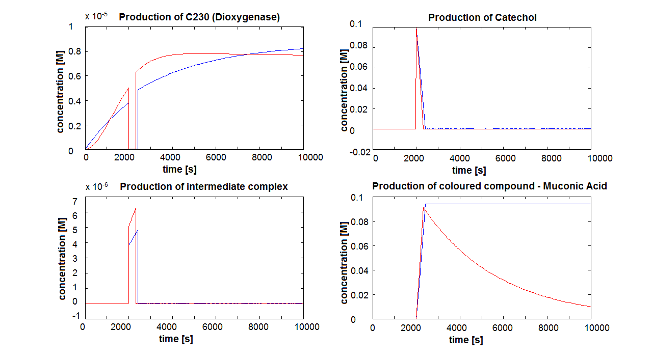
|Colour response model for cells being kept alive. | |Colour response model for cells being kept alive. | ||
|} | |} | ||
</div> | </div> | ||
| - | + | ||
| + | <div ALIGN=Center> | ||
{| style="width:395px;background:#e7e7e7;text-align:center;font-family: helvetica, arial, sans-serif;color:#555555;margin- top:5px;padding: 1px;" cellspacing="5"; | {| style="width:395px;background:#e7e7e7;text-align:center;font-family: helvetica, arial, sans-serif;color:#555555;margin- top:5px;padding: 1px;" cellspacing="5"; | ||
|- | |- | ||
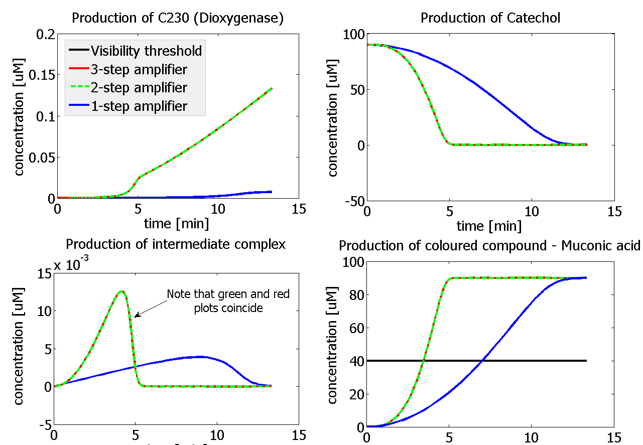
| - | |[[Image:IC_dead_cells.png| | + | |[[Image:IC_dead_cells.png|700px]] |
|- | |- | ||
|Colour response model with the same parameters for cells being killed instantaneously by catechol. | |Colour response model with the same parameters for cells being killed instantaneously by catechol. | ||
|} | |} | ||
</div> | </div> | ||
| - | |||
<html><h3>References</h3> | <html><h3>References</h3> | ||
Revision as of 16:43, 26 October 2010
| Modelling | Overview | Detection Model | Signaling Model | Fast Response Model | Interactions |
| A major part of the project consisted of modelling each module. This enabled us to decide which ideas we should implement. Look at the Fast Response page for a great example of how modelling has made a major impact on our design! | |
| Objectives | Description | Results | Constants | MATLAB Code |
| Results | |||||||||||||||||||||||||||
| During the construction of the model and after the whole models were completed they were tested and their behaviour observed and analysed. The most common method that we used for analysing our models was parameter analysis. This involves taking one particular parameter, varying it across several orders of magnitude and observing the results. This was important during the development of the models so that we could determine which parameters our models are most sensitive to. Then efforts would be made to determine these paramteres in the labs or take extra care in looking for them in research papers. In order to see the parameter sensitivity analysis results click on the button below:
Parameter Sensitivity Analysis
1. Parameter sensitivity performed on penultimate amplification levelThe observations below are based on models that were implemented up to the production of dioxygenase. Catechol was not added to the system, so conclusions are based on the concentrations of dioxygenase. The results of the full models, including the colour output, are included in section 2 below. Challenges Despite being quite thoughtful in translating our models into MatLab, unexpected outputs were observed. For example, some species were generating negative concentrations. In particular, for initial dioxygenase concentrations smaller than 10-4 mol/dm3 the results were inconclusive since they were oscillating around zero. We realised that this could be due to the ode-solver that we were using initially (ode45 in Matlab). Trying to correct this problem with the ode-solver, the following precuations were implemented:
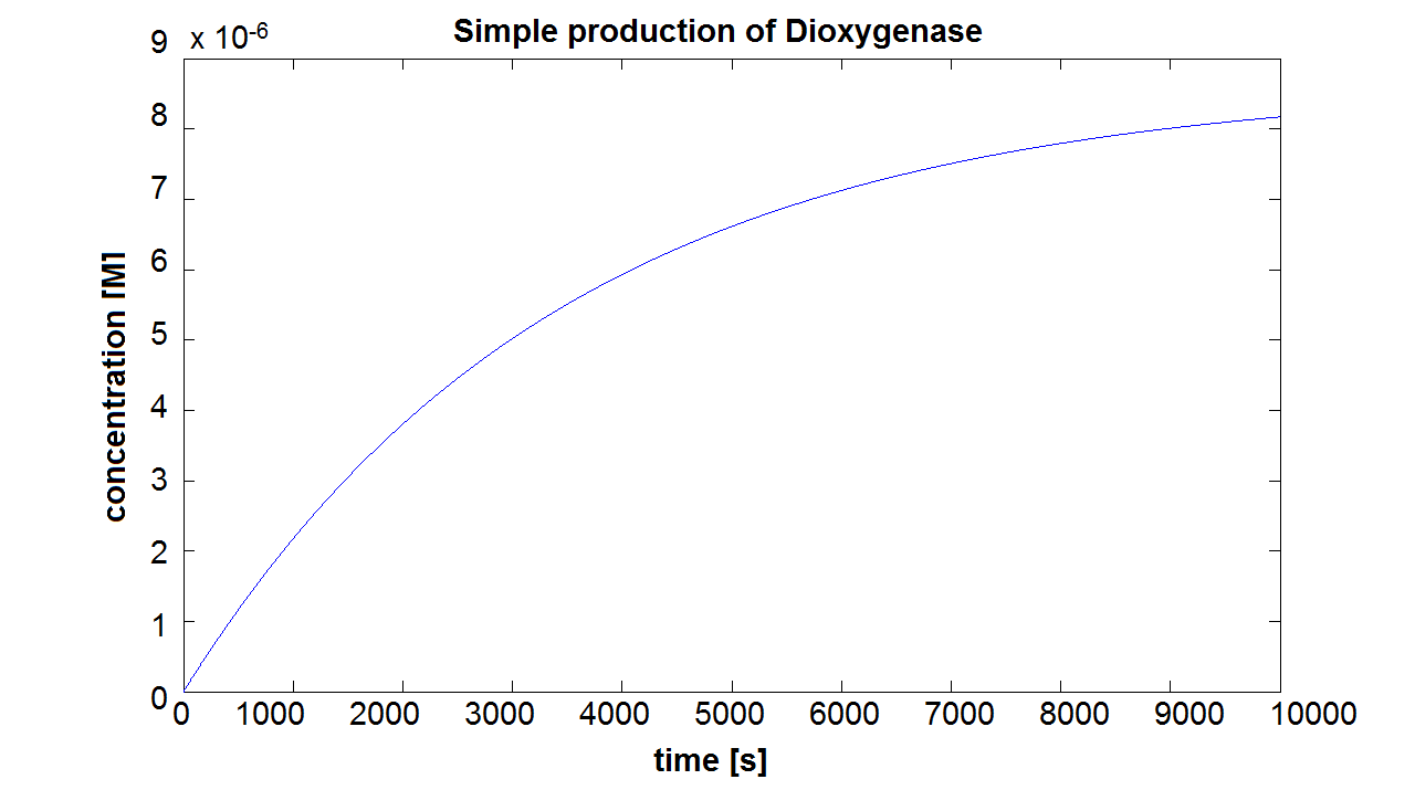
When we entered the real production and degradation rates into our model, we again obtained negative values. This was due to our set of differential equations being stiff. Since ode45 cannot solve stiff differential equations, we had to switch to using ode15s - an ODE-solver designed to handle stiff equations. Model pre-A This is the result of the simulation of simple production of Dioxygenase. It can be seen that the concentration will tend towards a final value of approximately 8×10⁻⁶ mol/dm3. This final value is dependent on the production and degradation rate(which has been estimated for all of the models). On the website E.coli Statistics [http://gchelpdesk.ualberta.ca/CCDB/cgi-bin/STAT_NEW.cgi] it is stated that number of ribosomal proteins per cell is 900,000. In a cellular volume of order of 1μm3 = 10-15dm3=10-15L, the above number of ribosomes converts to 1.5×10⁻³mol/L. This means that a concentration of 10-5mol/dm3 is not out of scale and there is even some room for manipulation. Sensitivity of Model preA
Model A Sensitivity of Model A We want to determine how our system reacts if different parameters are changed. This is to find out which parameters our system is very sensitive to.
Hence, the system is sensitive to most of the constants (given a particular range of values). The most crucial one, however, seems to be the initial concentration of split Dioxygenase and kcat. Model B Sensitivity of Model B This model has shown very similar sensitivity results as Model A, eg.:
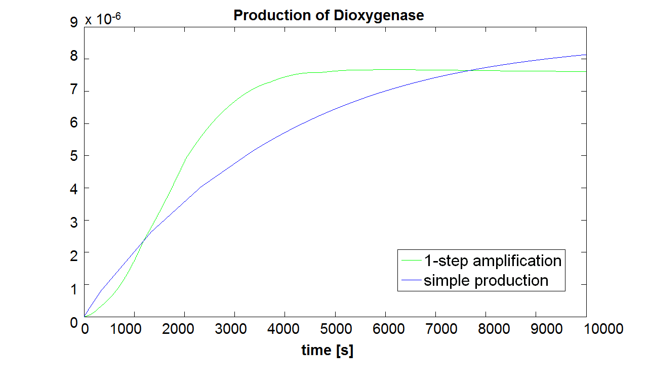
The initial concentration of split Dioxygenase, c0, determines whether the system is amplifying. Model A vs. B Running both models with the same initial conditions (c0=10-5 mol/dm3),it has been noted that Model B does not generate a siginificant amplfication over Model A. Hence, it would be more sensible to integrate a one step amplification module into our system. 2. Paremeter sensitivity prformed on the complete modelsThe important information about the coloured compound (i.e. the product of the last enzymatic reaction) is toxic to the cells ([http://www.sciencedirect.com/science?_ob=MImg&_imagekey=B6V78-4XXNV4Y-4-7&_cdi=5836&_user=217827&_pii=S0048969709011668&_orig=search&_coverDate=02%2F01%2F2010&_sk=995919994&view=c&wchp=dGLbVzz-zSkzk&_valck=1&md5=f8dca6227c29db659ddbeb588ad115e7&ie=/sdarticle.pdf],[http://www.msk.or.kr/jsp/downloadPDF1.jsp?fileName=393-15.pdf]). It is suggested that product of by-product of catechol-dioxygenase reaction destroys the cell membrane by inhibiting lipid peroxidation. It causes significant changes in the structure and functioning of membrane components (e.g. disruption of membrane potential, removal of lipids and proteins, loss of magnesium and calcium ions). These effects cause the loss of membrane functions, leading to cell death. In order to determine as least qualitatively the influence of cell death on performance of the amplifiers, 2 versions of models have been designed. Once version is neglcting the cell death while the other models instantaneous cell death with addition of catechol. Cell death in our models means that production of any proteins stops, but the reactions are still allowed to perform. Challenges Once we have implemented the colour change into the models, we noticed that there are some odd results. After adding catechol, some concentrations were reaching negative values. We checked our equations and constants but could not find a mistake. Hence, we concluded that there must be something wrong with the way that MatLab evaluates the equation or deals with the numbers. The problem seems to originate from the very rapid concentration change of catechol which disrupts the whole system. Tried solutions:
We hoped that TinkerCell imposes non-negative conditions on its solutions. Hence, we implemented the whole amplification model (including coloured output) in TinkerCell. However, we realized that TinkerCell does not deal well with very high or low numbers (For example, values higher than 105 are not acceptable - this is important since our rate constants (k1) are usually bigger than 105. Also, the low degradation rates (10-9) result in a zero output line). However, TinkerCell can still be used for testing that our Matlab programs behave the way we anticipated (by using default parameter values of 1), as well as producing illustrative diagrams of our system.
We had a close look at the ODE solver options in MatLab. However, we were already using the one that produced the most reasonable results (ode15s). We found that decreasing Relative and Absolute tolerances (to values as small as 10-15) significantly improved the simulation. However, this is not an ultimate solution as in the simulations negative numbers still appear (order of 10-15). We decided that such small negative concentrations were acceptable. We also decided that the point of interest lies between the first 100 to 150 seconds after adding catechol, while concentrations hit the negative values at much higher time values. The images below show the influence of the relative and absolute tolerance values on the model. Note that it was important to allow the ODE-solver to adjust the time step automatically, as big time steps (1 second) were generating wrong answers for the catechol model. Adjusting time steps manually to very small values was not efficient (the whole simulation does not require very high definition simluation).
We hoped that SimBiology could be more suited for our modelling than using ODE-solvers, so we implemented our models into SimBiology. This package offers an interactive user interface similar to Tinker Cell, but uses MatLab to simulate. Initially, we confirmed that our simple production model (Model PreA) and 1-step amplification model (Model A) implemented in SimBiology generated exactly the same results as our ODE equation based models. The interface allowed us to have clearer control over parameters. It also allowed modelling special events, for example, adding catechol at certain point in time. Previously we had to split simulation into to two parts. Conclusions
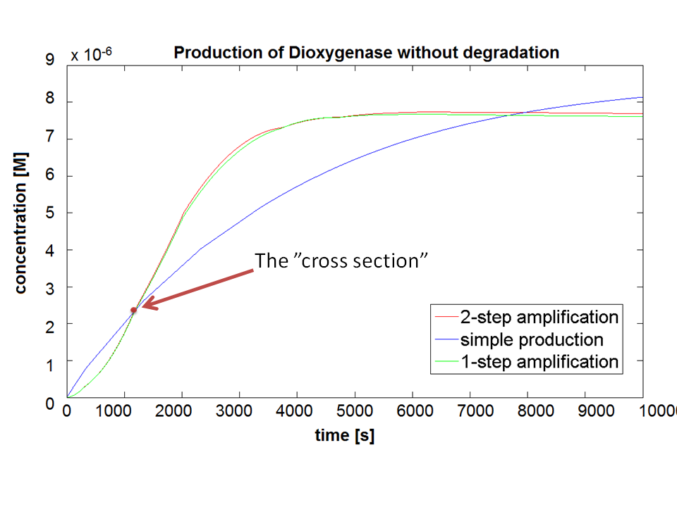
If Catechol is added before t= 500s, then the coloured output will reach its threshold value faster by 1-step amplification. If Catechol is added when t>500s, then the coloured output will increase (marginally) faster through the amplification step in Model A (2-step amplifier). However, then there does not seem to be a appreciable difference between the two models (Model preA and Model A). These observations are true for intial concentration of dioxygenase equal to 10-5mol/dm3. However, we noticed that if the initial concentration is raised to 10-4mol/dm3, then Model A can be more beneficial than Model preA after only 100 seconds. Note that time of adding catechol does not exactly correspond to “cross-section” in Figure 3 as the systems still work after adding catechol, so it can be added a bit before the “cross section”. However, there is no point in delaying addition of catechol into system just prove that 2-step amplification could work.
There seem to be 3 regions of catechol concentration that influence the system in different ways. Whatever, the initial conditions and other parameters are, those 3 regions exist, but their boundaries move around. For one particular sequence of initial conditions, these regions were: c>1M, 1M>c>0.01M, 0.01M>c. Varying the initial concentration of catechol within the highest region does not result in any change of colour output response (It is possible that all enzymes are occupied and the solution is over saturated with catechol). In the middle region the catechol concentration influences the amplfication. Amplification decreased when the concentration tends towards the 0.01M border. When the lowest region is entered, there is no difference in output production by Model A and preA.
The coloured product of catechol kills cells by destroying the cell membrane. However, we do not know how quickly the cells will die. Therefore, we examined two different cases: immediate cell death and negligible cell death (i.e. cells death is negligible because it takes too long) Running the simluation in Matlab (not Simbiology!), our conclusions are:
Since it appears that the time of cell death is important, we decided to discuss this issue with our team members. Referring to this paper [1] we decided that cell death induced by catechool is a very slow process (we estimate that it will take a few hours) in comparison to the time scale that we are interested in (several seconds to minutes). Hence, our final conclusions will be on the model neglecting cell death. References
|
| Conclusions | ||
Having explored the sensitivity of our models at 2 amplification levels and after many values were constrained by lab results or biological ranges, 2 parameters have been recognised as crucial. Their values are decisive regarding the design of the 1 and 2 output amplification systems. Hence, one should pay most attention to them, when trying to assemble similar systems:
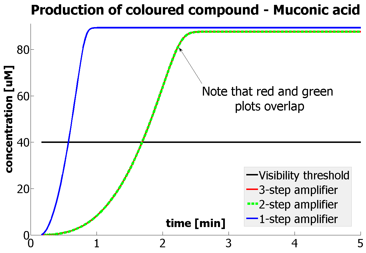
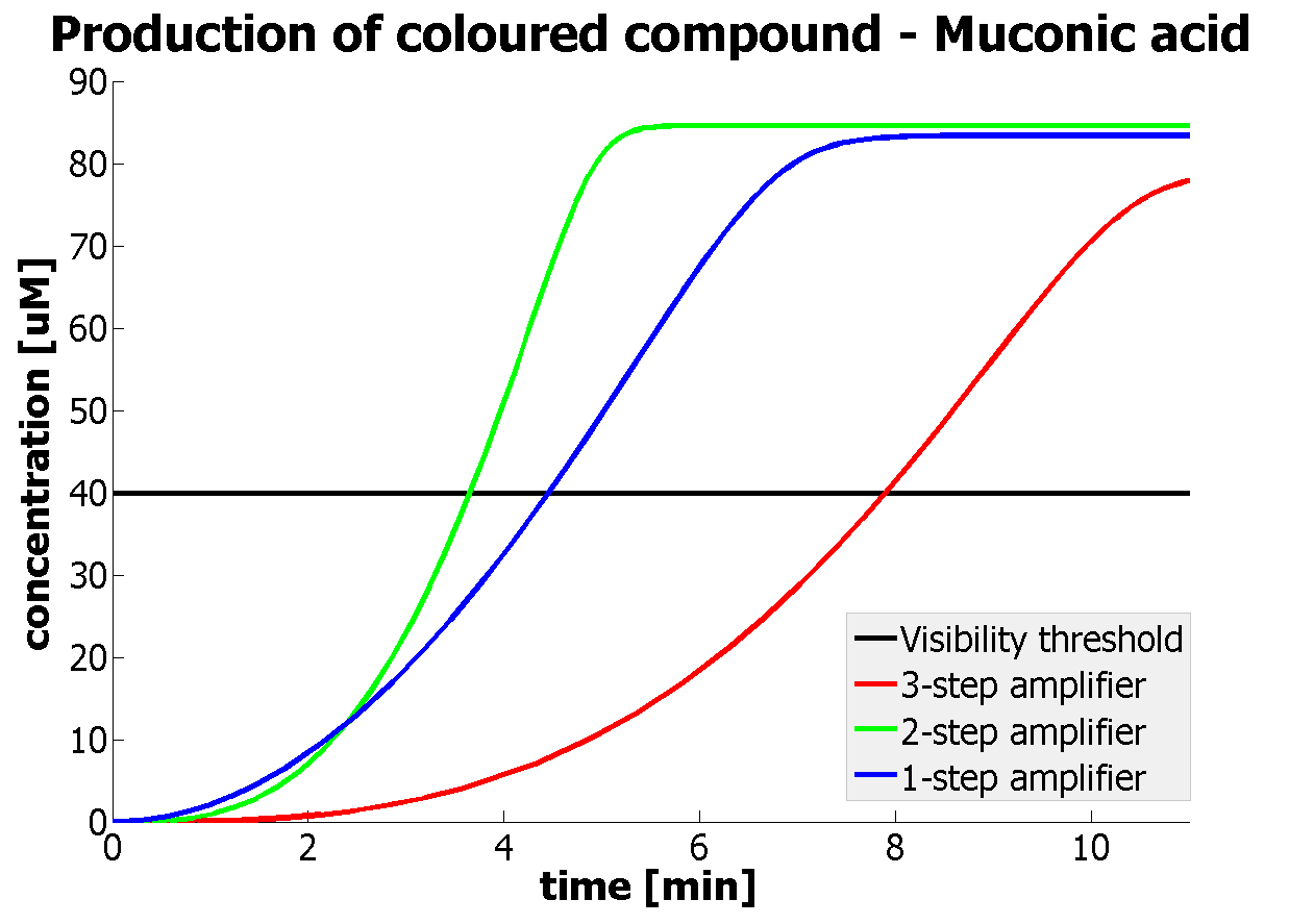
This is one of the parameters that could have been very poorly estimated in our models. Initially, all our models have been tested for values which we thought could correspond to high copy plasmids in E.Coli (rate= 2.4998×10⁻⁹ M/s). 2 step-amplification performs worse than 1-step amplification given biologically relevant concentrations of catechol (and considering other constraints). However, our system is implemented in Bacillus subtilis which expresses genes very weakly. If its expression rate of dioxygenase is 1 or 2 magnitudes lower than in the case of E.Coli, then 2-step amplification seems to be 4 minutes faster than 1-step amplification (see figure below).
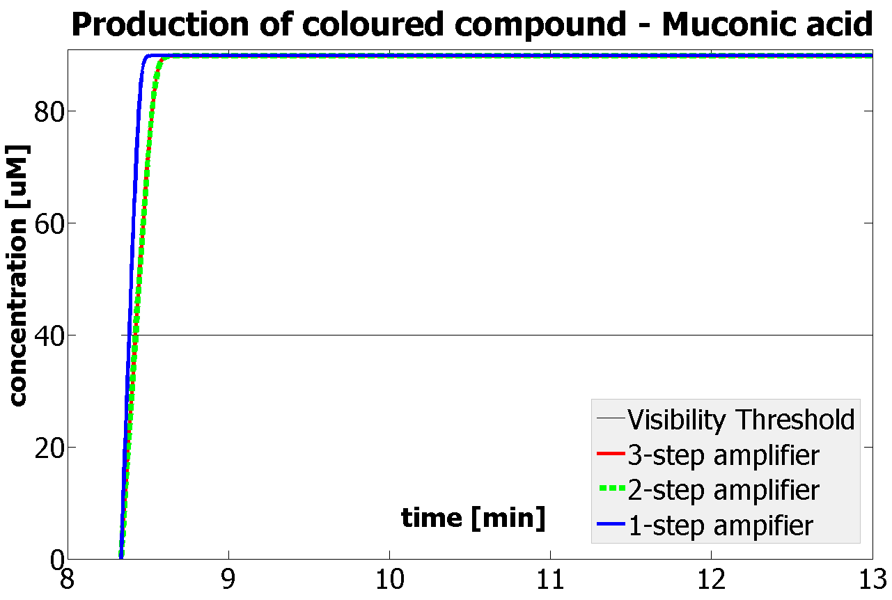
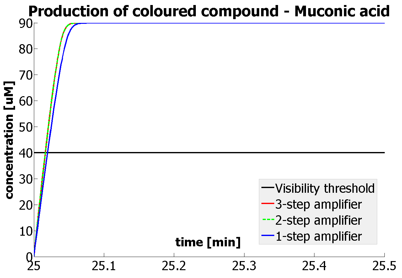
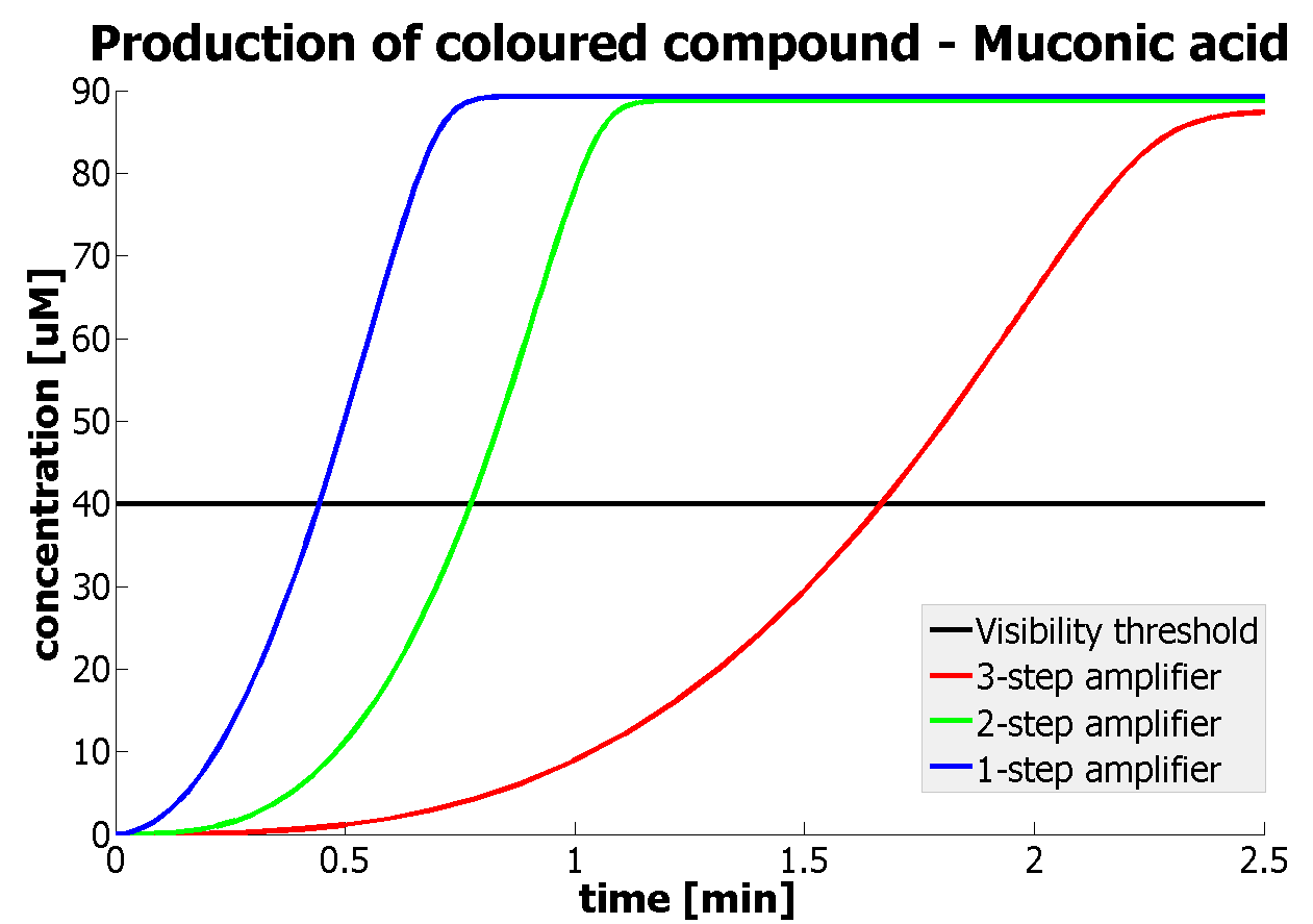
It should be noticed that kcat of Dioxygenase (kcat=52) is 4 magnitudes higher than kcat of TEV (kcat=0.16) . This is a tremendous difference and it emphasises the efficiency of the 1-step amplifier. Basically, in our combination of enzymes the second one – TEV – does not have much to improve on. It is even harder for 2-step amplifier to be efficient taking into account the slow action of the TEV protease. To analyze the importance of the kcat values please observe the graphs below. From the above graphs it can be seen that if the situation regarding kcat values was reversed 2-step amplifier would perform much better than the 1 step amplification system even for high copy plasmids like E.Coli! Clearly, 3 step amplification does not perform well under the given conditions, due to too much delay being introduced by the third amplification step. Hence, if one was to design the amplification module for different colour outputs and would not be satisfied with the speed of response generated by 1-step amplification, it would be recommended to choose the first enzyme 1 (refer to picture below) to have a kcat value that is at least 2 magnitudes higher than the kcat value of enzyme 2 (for high expressing chassis).
The two factors can decide whether the 2-amplifier system could perform better than the 1-step amplifier. The effect of these two factors can be combined to generate even more efficient systems. If one was using a chassis of medium expression rate, then choosing enzymes with 1 magnitude difference in kcat would result in the 2-step amplifier performing better. |
 "
"


