"

From 2010.igem.org

Modelling

Wiring Diagram

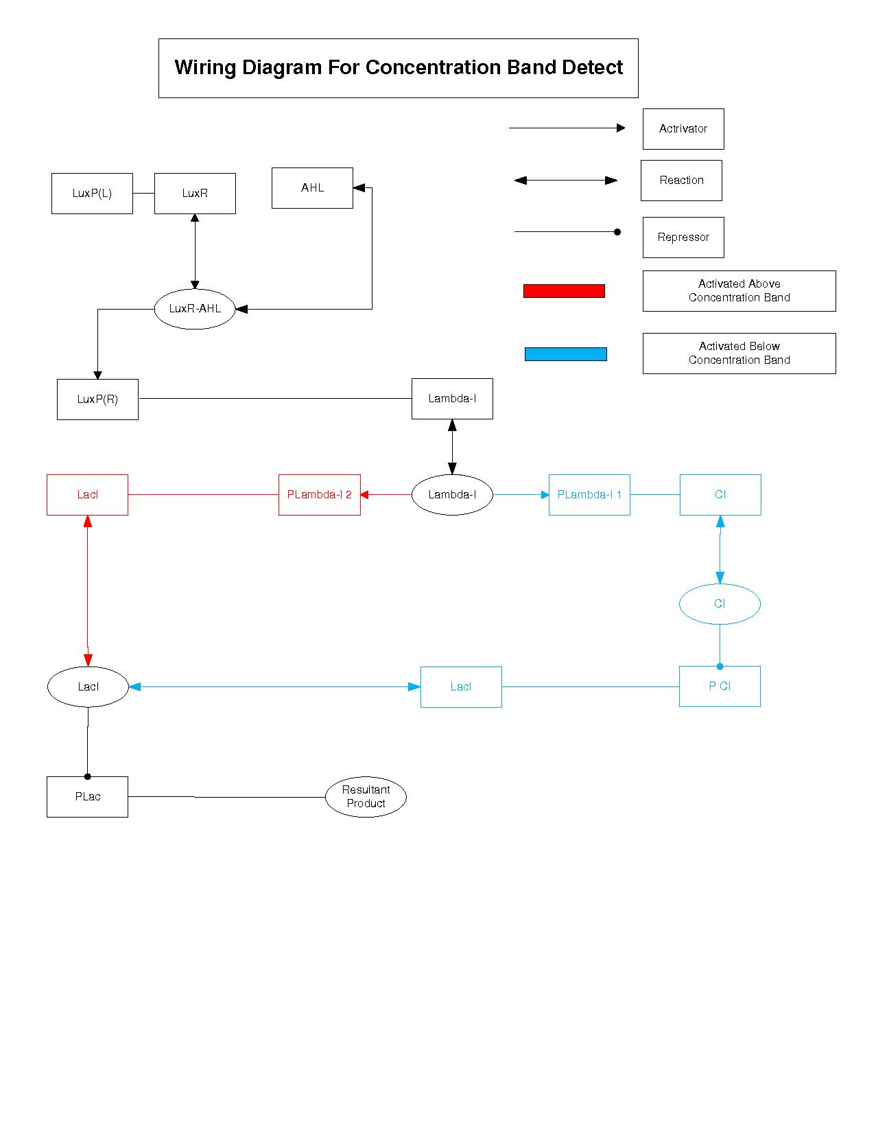
This is a outline of the regulatory topology of the concentration band-detect architecture.The different components and the way they interact with each other is represented similar to a electronic circuit.We use this as the starting point for building our model.First each of the components of our system was mathematically formulated. The components were then put together to form the whole system.

Model

Based on the network diagram above, equations were written for each of the steps in the pathway. To keep the system simple, terms for degradation and synthesis were setup as given below:

dlam=((k1*(ahl/km1)^n1)/(1+(ahl/km1)^n1))-k2*lam;

dahl=0;

Assuming a constant amount of AHL input. However, we check the response of the system for different concentration of AHL.

dci=((k3*(lam/km3)^n2)/(1+(lam/km3)^n2))-k4*ci;

The equations follow the simple mechanism of activator and repressor kinetics.

dlaci=(k5/(1+(ci/km3)^n3))+((k6*(lam/km4)^n4)/(1+(lam/km4)^n4))-k7*laci;

dgfp=(k8/(1+(laci/km5)^n5))-k9*gfp;

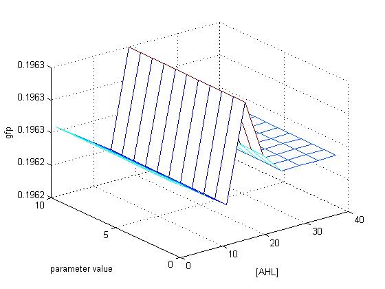
The final equation is a measure of the response of the system to different amounts of input signal.

Results

Code

odeIGEM03.m

 %lambda1 function file

function dX =odeIGEM02(t,X,P)

k1=P(1);

k2=P(2);

k3=P(3);

k4=P(4);

k5=P(5);

k6=P(6);

k7=P(7);

k8=P(8);

k9=P(9);

k10=P(10);

k11=P(11);

km1=P(12);

km2=P(13);

km3=P(14);

km4=P(15);

km5=P(16);

ahl=X(1);

lam=X(2);

ci=X(3);

laci=X(4);

gfp=X(5);

n1=1;

n2=1;

n3=1;

n4=1;

n5=2;

dlam=((k1*(ahl/km1)^n1)/(1+(ahl/km1)^n1))-k2*lam;

dahl=0;%k10*ahl-k11*ahl;

dci=((k3*(lam/km3)^n2)/(1+(lam/km3)^n2))-k4*ci;

dlaci=(k5/(1+(ci/km3)^n3))+((k6*(lam/km4)^n4)/(1+(lam/km4)^n4))-k7*laci;

dgfp=(k8/(1+(laci/km5)^n5))-k9*gfp;

dX=[dahl dlam dci dlaci dgfp]';

Main.m

%Comment %Date:28th July 2010

A=linspace(1,40,10);

p=linspace(1,10,11);

G=zeros(length(A),length(p));

B=linspace(1,40,10);

q=linspace(1,10,11);

C=linspace(1,40,10);

r=linspace(1,10,11);

v=15;

%Initial Conc.

lam=0;

ahl=1;

ci=0;

laci=0;

gfp=0;

k1=60;%first case used 1;second case used 30;%third case use 60

firstk1=1;

secondk1=30;

thirdk1=60;

k2=0;

k3=0.2;%first case used 10;second case use 0.98;third case use 0.2

firstk3=10;

secondk3=0.98;

thirdk3=0.2;

k4=0;

k5=1;

k6=0.001;

k7=0;

k8=2;

k9=10;

k10=0;

k11=0;

km1=0.5;

km2=0;

km3=1;

km4=0;

km5=40;

X0=[ahl,lam,ci,laci,gfp]';

%parameters

%P=[k1 k2 k3 k4 k5 k6 k7 k8 k9 k10 k11 km1 km2 km3 km4 km5]';

firstP=[firstk1 k2 firstk3 k4 k5 k6 k7 k8 k9 k10 k11 km1 km2 km3 km4 km5]';

secondP=[secondk1 k2 secondk3 k4 k5 k6 k7 k8 k9 k10 k11 km1 km2 km3 km4 km5]';

thirdP=[thirdk1 k2 thirdk3 k4 k5 k6 k7 k8 k9 k10 k11 km1 km2 km3 km4 km5]';

tspan=linspace(0,10,1e3); %linspace(start time,finishing time, number of steps)...

opt=odeset('Abstol',1e-13);

%for j=1:length(A)

% for i=1:length(p)

%       P(v)=p(i);
       
%       X0(1)=A(j);
       
%       [t X]=ode15s(@odeIGEM03,tspan,X0,opt,P);
       
%       G(j,i)=X(end,5);

%   end

%end

%[A p]=meshgrid(A,p);

%mesh(A,p,G')

for j=1:length(A)

   for i=1:length(p)
       
       firstP(v)=p(i);
       
       X0(1)=A(j);
       
       [t X]=ode15s(@odeIGEM03,tspan,X0,opt,firstP);
       
       G(j,i)=X(end,5);

   end

end

[A p]=meshgrid(A,p);

mesh(A,p,G');

figure;

for j=1:length(B)

   for i=1:length(q)
       
       secondP(v)=q(i);
       
       X0(1)=B(j);
       
       [t X]=ode15s(@odeIGEM03,tspan,X0,opt,secondP);
       
       G(j,i)=X(end,5);

   end

end

[B q]=meshgrid(B,q);

mesh(B,q,G');

figure;

for j=1:length(C)

   for i=1:length(r)
       
       thirdP(v)=r(i);
       
       X0(1)=C(j);
       
       [t X]=ode15s(@odeIGEM03,tspan,X0,opt,thirdP);
       
       G(j,i)=X(end,5);

   end

end

[C r]=meshgrid(C,r);

mesh(C,r,G')

xlabel('[AHL]')

ylabel('parameter value')

zlabel('gfp')