Team:TU Delft/Project/rbs-characterization/characterization
From 2010.igem.org

Characterization
By varying only the RBS sequence in a protein generator construct the dependence of the expression level of the encoded protein on the RBS sequence could be determined by simple fluorescence and biomass curve analysis. The methods are further explained below.
What is this 'strength' we are attempting to characterize?
In the field of synthetic biology the 'strength' of an RBS is defined as the rate at which translation is initiated by the RBS sequence on any given mRNA molecule. Going back a step, we see that translation initiation occurs preferentially at certain mRNA sequences, which show a similarity to the consensus -Shine-Delgarno- sequence. This is due to the optimal binding of the 16S rRNA at these regions. In other words, the RBS 'strength' may loosely be defined as the rate of ribosome binding to any given mRNA molecule. (Click here for more information.)
For our project it is not directly the binding equilibria of ribosome to mRNA that is of interest to us, but rather the netto rate of protein production. Thus, in our experimentation we define the RBS strength as the production rate of a given protein downstream of an RBS.
The experimental method
The E.coli strains carrying the parts to be tested were cultured for 16 hours on 96-well plates while measuring fluorescence of GFP and biomass absorbance at 10 minute intervals. Click [here] for the more detailed protocol.
Previous methods
We've seen that previous teams have performed their protein expression rate analysis to only include current protein level (fluorescence measurements) and current biomass concentration (absorption measurements). However, we've found that during measurements, the protein concentration is also influenced by other factors:
- The rapid growth of the bacteria dilutes the protein considerably
- Proteins degrade over time.
The conventional method for characterization of RBS or promotor sequences is to assume that the derivative of the GFP fluorescence is equal to the production rate, as shown in the formula from Kelly et al [1].

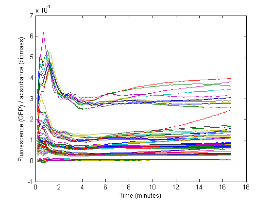
However, this method would only be representable if the strains are subcultured a multiple times from the exponential phase. In that case, a steady state GFP concentration (fluorescence) may be assumed and dilution is ignored. Due to the decrease in the biomass specific GFP fluorescence at the start of the measurements it was assumed that dilution effects played an important role in our data and thus was taken into account for our model.
Growth curve fitting
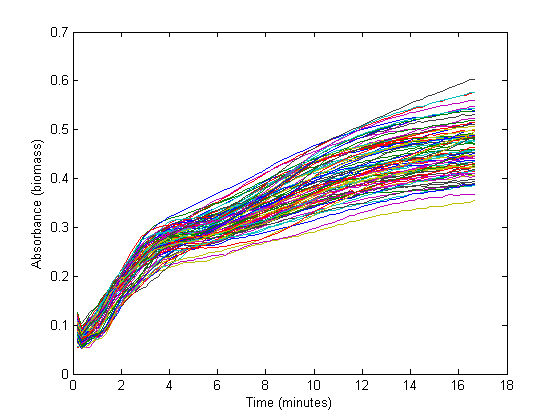
From the biomass, or optical density (OD), graph below, it can be seen that the fastest growth occurs from 1 hour until about 3 hours into the experiment. Within this timespan, it is assumed that growth is exponential, and growth rate can be calculated. The graph below shows 72 growth curves. 12 seperate wells were used for every RBS sequence.
The exponential part of this graph is curve-fitted to an exponential growth model:
Which results in a growth rate ('mu') that can be used to add dilution to further calculation.
Biomass growth will dilute the GFP
At the start of our measurements, the GFP protein has reached a steady state high concentration. The specific GFP will decrease during growth because of dilution, and this needs to be accounted for when calculating the RBS strength.
Protein production model
As said, the protein production model needs to take dilution into account. The GFP protein that is used is very stable (half life 41 hours), so the degradation term is negligible compared to dilution.
In above formula:
- Y is the GFP concentration
- Beta is the production rate (The constant that we are interested in)
- Alpha is the dilution+degradation rate
Converting this equation to an explicit form results in:
The 2 unknown parameters (beta and Y1) where curve-fitted against the GFP/OD data, using the matlab lsqcurvefit command. The beta constant for each of the 72 experiments were then to calculate RBS strengths, listed in the results page.
Data normalization method
To go from original measurements to RBS strenghts, we ran the following steps using a matlab script:
Our plate reader data consists of 12 columns of
- 5 strains with Anderson RBS'es to be characterized
- B0032 strain to compare to
- I13401 strain as control (GFP without promotor and RBS)
- LB+Amp as blank
To prepare the data for further calculation, some things have to be done:
- Subtract the blank GFP and OD values from the data with E coli in it. This takes care of the platereader error independent of biomass
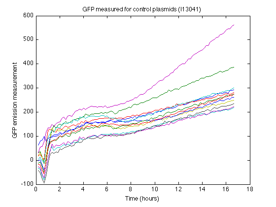
- Biomass without GFP also produces some nonzero measurements (See right). From the control strain measurements we can calculate how much 'fake' GFP is reported due to biomass.
- For each well, we calculate the real GFP that is not a result of biomass:
real_gfp = gfp - fake_gfp_per_od * od
- These values are curve fitted into our protein production model, resulting in a (exponential phase) protein production rate for each well.
Source code and data
https://static.igem.org/mediawiki/2010/8/88/TUDelft_2010_RBS_characterization.zip
References
[1] Jason R. Kelly, Adam J. Rubin, Joseph H. Davis, et al (March 2009). "Measuring the activity of BioBrick promoters using an in vivo reference standard". Journal of Biological Engineering 3: 4

 "
"


