Team:BCCS-Bristol/Modelling/GRN/Results
From 2010.igem.org
m |
|||
| Line 11: | Line 11: | ||
[[Image:AgrEcoli_phase_plane.jpg|frameless|center|upright=4|Phase Plane of agrEcoli GRN with level curves]] | [[Image:AgrEcoli_phase_plane.jpg|frameless|center|upright=4|Phase Plane of agrEcoli GRN with level curves]] | ||
| + | |||
| + | A two-dimensional phase plane diagram is a useful way of showing the dynamics of a system. The phase plane diagrams below show the rate of change of NsrR and GFP given the current quantity of each. This is shown as arrows on a plane, with the direction of the arrow signalling increase or decrease of a variable, and the size of the arrow describing the magnitude of the change. Also plotted on the diagram are level curves (blue). These represent the specific trajectory of some given initial conditions. Level curves are very useful to visualise a range of initial conditions. | ||
| + | |||
| + | This diagram shows that a single stable solution exists, and that all trajectories converge to it eventually. This is unsurprising, as GFP, NsrR and mRNA all break down naturally. Therefore it makes sense that for any fixed production rate of any of these proteins, there will exist some point at which the rate of breakdown matches the rate of production, and the system reaches equilibrium. It is useful to confirm the existence of an equilibrium point mathematically, and locate it as a function of the constants in the equations. This allows predictions to be made about the behaviour of the system over time, avoiding the need for explicit experimental verification. | ||
Revision as of 17:32, 24 October 2010
iGEM 2010
Results
Phase Planes
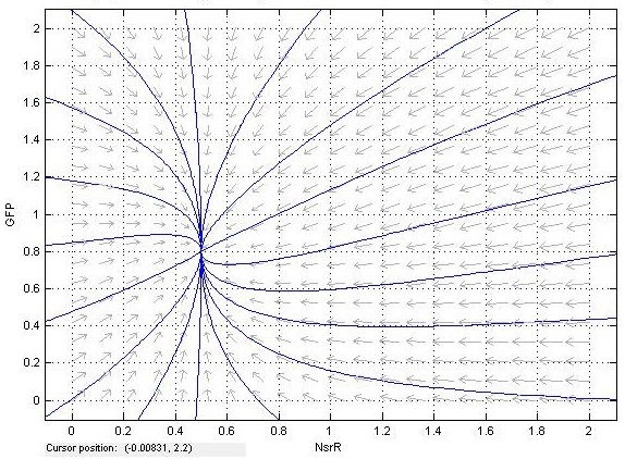
A two-dimensional phase plane diagram is a useful way of showing the dynamics of a system. The phase plane diagrams below show the rate of change of NsrR and GFP given the current quantity of each. This is shown as arrows on a plane, with the direction of the arrow signalling increase or decrease of a variable, and the size of the arrow describing the magnitude of the change. Also plotted on the diagram are level curves (blue). These represent the specific trajectory of some given initial conditions. Level curves are very useful to visualise a range of initial conditions.
This diagram shows that a single stable solution exists, and that all trajectories converge to it eventually. This is unsurprising, as GFP, NsrR and mRNA all break down naturally. Therefore it makes sense that for any fixed production rate of any of these proteins, there will exist some point at which the rate of breakdown matches the rate of production, and the system reaches equilibrium. It is useful to confirm the existence of an equilibrium point mathematically, and locate it as a function of the constants in the equations. This allows predictions to be made about the behaviour of the system over time, avoiding the need for explicit experimental verification.
 "
"

