Team:ETHZ Basel/Modeling/Movement
From 2010.igem.org
(→Variations in input bias) |
m (→Direction changes) |
||
| Line 42: | Line 42: | ||
==== Direction changes ==== | ==== Direction changes ==== | ||
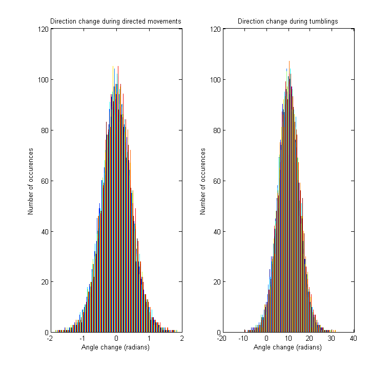
| - | [[Image:ETH_iGEM_angle_distribution.PNG|thumb|300px| '''Changes in movement angle during chemotaxis movement''' Probability distributions from which the angle changes are sampled. Left figure: Directed movement state. Right figure: Tumbling state ]] | + | [[Image:ETH_iGEM_angle_distribution.PNG|thumb|300px| '''Changes in movement angle during chemotaxis movement''' Probability distributions from which the angle changes are sampled. Left figure: Directed movement state. Right figure: Tumbling state. ]] |
The tumbling angle is the change of direction between two directed movements. Since we are working with a continuous model, the derivative of the angle (i.e. angular velocity) is sampled for every tumbling, from a distribution resembling the empirically observed one [[Team:ETHZ Basel/Modeling/Movement#References|[1]]]. | The tumbling angle is the change of direction between two directed movements. Since we are working with a continuous model, the derivative of the angle (i.e. angular velocity) is sampled for every tumbling, from a distribution resembling the empirically observed one [[Team:ETHZ Basel/Modeling/Movement#References|[1]]]. | ||
<br> | <br> | ||
Revision as of 15:55, 24 October 2010
Modeling & Simulating Bacterial Movement
Overview
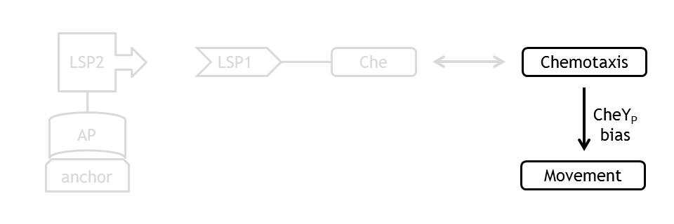
Analogous to the highly complex signal transduction network in the chemotaxis receptor model, there is an equally challenging molecular mechanism on side of the flagella, responsible for the movement of the bacterium.
In order to capture the features of cell motility, we implemented a probabilistic model, which simulates the cell movement in accordance to the existing empirical observations. Different from the molecular model, which operates in continuous time, the cell motility model operates with a fixed time step, which can however be adjusted arbitrarily. For our simulations we have chosen a timestep Δt=0.03s, which is around five times smaller than the smallest time constants in the cell motility model as well as over ten times smaller than the time constant with which the CheYp concentration changes in the molecular model (see Section Experimental Design.
At every time step of the simulation of the cell motility model, the current CheYp concentration is received as an input from the chemotaxis pathway model. This input determines the probability of the CCW and the CW rotation direction of the flagellums. A counterclockwise rotation corresponds to the directed movement (running) state and to a change in spatial coordinates, together with a slight change in angle, while a clockwise rotation corresponds to the tumbling state and to a new movement direction, with nearly unchanged other spatial coordinates.
By coupling the probabilistic movement model with the deterministic molecular model we can realistically simulate the variations in motility which occur due to variations in the concentrations of the molecular species of the chemotaxis pathway, namely in the concentration of CheYp.
Algorithm
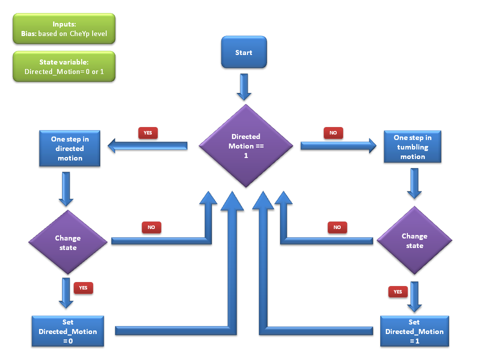
We use a two state model that reflects the two states the cell can be in through out its motion - swimming state & the tumbling state. At each time-step of the simulation, the cell will either stay in the same state or will switch the state according to these probabilities. Details of these probability values can be found below.
In each of these states, there is a transition probability to switch to the other states as described above. (We have the probability P1 that tells us the probability of switching to the tumbling state when the cell is currently in the swimming state and also the probability P2 that that reflects the probability of switching to the running state). At each timestep of the algorithm, the decision whether to run or tumble in the next timestep is taken based on these two probabilities.
If the decision was to run in the next timestep, the cell will be moved to it's next point with a velocity that agrees with literature [1]. Also, there is a slight deviation in the angle it moves during running. This angle is much smaller than the angle change during a tumbling timestep & it is sampled from a distribution that is suggested based on empirical data [1].
During a tumbling timestep, the angle of tumbling is decided such that the tumbling angle (between two directed motion segments) is a Weibull distributed random variable as suggested in [1].
We have made sure that the movement simulated using the algorithm agrees with the observed behaviour of E. coli in chemotaxis motion.
Concepts
The main concepts we used in deriving and implementing our model are based on the most important features observed in the real behavior of E. coli. These features are:
Bias
The quantity that links the CheYp concentration with the type of motion (tumbling vs. directed motion) is called the bias and it is formally defined as the fraction of time spent in the directed movement state with respect to the total time in motion. Our choice for bias formulation was a nonlinear Hill - type function of CheYp concentration, with one of the parameters being the wild-type CheYp concentration for which a steady - state invariant time ratio was obtained. Both the functional dependency and CheYp value are well documented in literature [2].

At every time point of the simulation, the cell probabilistically chooses whether to employ directed movement or to tumble, depending on the value of the bias (later described in the Algorithm subsection).
Mean times
An important way of characterizing the cell's behavior is by statistically observing it over a longer time period.
From this aspect, the mean tumbling length is the average time the cell spends in between two directed movement states, while the mean run length is the average time spent in the directed movement state.

Direction changes
The tumbling angle is the change of direction between two directed movements. Since we are working with a continuous model, the derivative of the angle (i.e. angular velocity) is sampled for every tumbling, from a distribution resembling the empirically observed one [1].
As stated above, the model allows direction changes also during directed movements periods. In contrast to the tumbling state, this angle change is much smaller, being drawn from a normal distribution with 0 mean and standard deviation obtained from the literature [1].
Since the cell can move either clockwise or couterclockwise at every step of the simulation, the angle and tumbling speed distributions are always symmetrical about 0.
This ensures a realistic simulation of bacterial movement, not only asymptotically, analyzed through statistical estimates, but also in each time - point, analyzed through individual changes in spatial coordinates and direction.
Transition Probabilities
One of the biggest challenges regarding the movement model was obtaining a time - step - invariant behavior of the cell, whose reliability of statistical estimates should be the same, regardless how often the cell had to choose its future state.
In order to achieve this, we opted for a two - state first - order Markov process, in which the future state is only dependent on the current state. Since we have boolean values for any possible state, we can define the following four transition probabilities, separately controlled depending on whether the cell is currently in the directive movement or in the tumbling state.

Therefore, the two central parameters of our model are the probabilities of keeping the current state also as future state: the probability that the future state is directed movement, when the current state is directed movement (p1) and probability of the future state being tumbling, when the current state is tumbling (p2).
In deriving the expression of these probabilities, we separately and symmetrically focused on the two processes: directed movement and tumbling. As a consequence, the mean run length is only dependent on the timestep and on the probability of continuing the directed movement (p1), while the mean tumbling length is only dependent on the timestep and on the probability of continuing tumbling (p2).
We will explain in detail the technique employed in deriving the probability of being in the directed movement state, when the previous state was directed movement. The symmetrical calculations, for the mean tumbling length, follow identically.
The mean run length is the expected value of a random variable representing the number of timesteps the cell consecutively spends in directed movement. By expanding the definition of an expected value, the mean run length becomes an infinite sum over all possible consecutive run-lengths, multiplied by their respective occurrence probabilities.
Assumptions
The assumptions of our model were taken in accordance with the existing experimental data on the chemotaxis movement [1]. The mean tumbling length was assumed to be constant, unlike the mean run length, which is a function of the bias. Besides the experimental evidence, this assumption also has a biological interpretation: tumbling is believed to occur because the flagella push each other away and disassemble after rotating counter-clock wise (directed movement). The duration spent in tumbling is a stochastic variable mainly representing the time the flagella afterwards need to reassemble, and a single process of reassembling is only weakly correlated with the frequency of tumbling.

Furthermore we assumed that the mean velocity during directed movements is constant and that the angle change during one tumbling block is constant.
Simulation Results
Variations in input bias
We simulated the spatial behavior of a single E. coli cell under the influence of different input bias values. For a more realistic simulation of the bacterial movement process, the input bias was obtained directly from the combined molecular model linking the chemotaxis pathway and the light switch. As the combined model offered us many design alternatives for performing simulations, we decided on a fixed molecular template, to ease the comparison of results.
The chosen molecular template for simulating the movement model was the following:
- molecular model chosen: Spiro et al [3]
- controlled Che species: CheY
- Light coupling: CheY-PIF3 & PhyB-Anchor
Each row of the subplots table presented below represents a different input bias value for the movement model, obtained as a result of different input protein concentrations for the combined molecular model. Each column represent a different simulation length (100 seconds, 500 seconds and 3000 seconds).
The input protein concentrations used, together with the corresponding obtained steady-state bias were the following:
All the simulations were run without the existence of any controller algorithm, therefore reproducing the random chemotaxis walk.
Please note the different spatial ranges when comparing the plots, increasing both with increasing simulation time length (the bacterium travels a longer distance in a longer time period) and with increasing bias value (the probability of choosing the directed movement state increases, therefore, on average, the cell travels a longer distance).
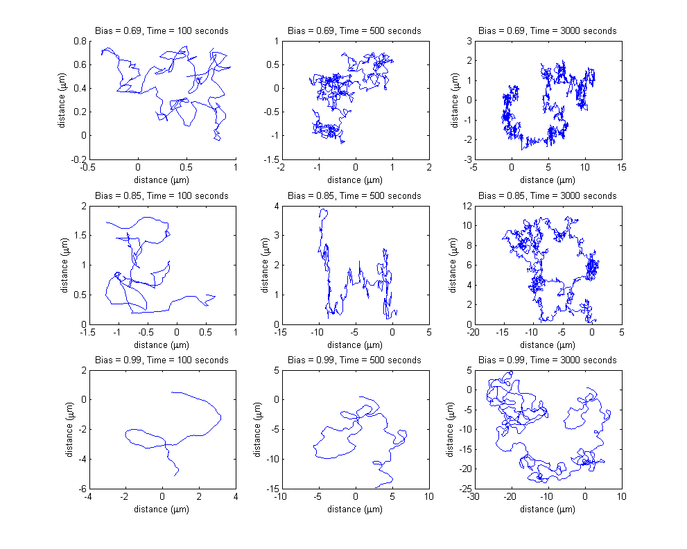
Please note the increasing axis range, both on the x and on the y coordinate, due to both increasing bias value and increasing simulation time.
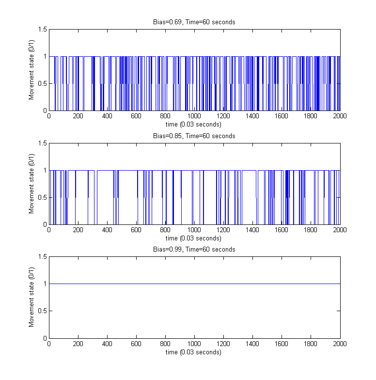
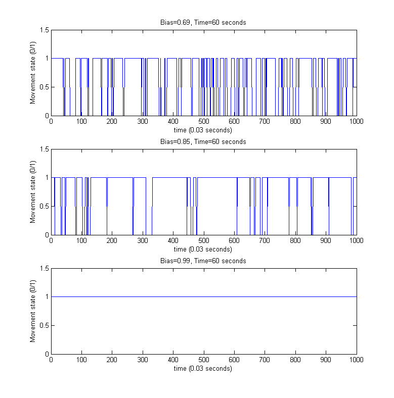
For the above simulated trajectories, we generated the so-called directed movement/tumbling plots used in analyzing chemotaxis motility from the perspective of boolean movement - time dependency. For providing a better visibility of the individual steps of the movement process, only the first 60 seconds of the above simulations were considered.
References
[1] [http://www.nature.com/nature/journal/v239/n5374/abs/239500a0.html H.C. Berg, D.A.Brown: Chemotaxis in Escherichia coli analysed by three - dimensional Tracking. Nature 1972 239, 500 - 504]
[2] [http://www.ncbi.nlm.nih.gov/pmc/articles/PMC1299372/?tool=pubmed Levin, Morton-Firth: Origins of Individual Swimming Behavior in Bacteria, Biophysical Journal 1998 74:175-181]
[3] [http://www.pnas.org/content/94/14/7263.full Spiro et al: A model of excitation and adaptation in bacterial chemotaxis. PNAS 1997 94;14;7263-7268.]
 "
"


