Team:ETHZ Basel/InformationProcessing/Controller
From 2010.igem.org
(→Threshold Optimized Controller (Winner of the Control Design Competition)) |
(→Four Zones of Preference Controller) |
||
| (15 intermediate revisions not shown) | |||
| Line 3: | Line 3: | ||
= Controller = | = Controller = | ||
| - | |||
[[Image:D1.png|thumb|400px|Block representation of the controller.]] | [[Image:D1.png|thumb|400px|Block representation of the controller.]] | ||
| + | |||
| + | <html><div class="thumb tright"><div class="thumbinner" style="width:402px;"> | ||
| + | <iframe title="YouTube video player" class="youtube-player" type="text/html" width="400" height="325" src="http://www.youtube.com/embed/z76qikmUKlo?rel=0&hd=1" frameborder="0"></iframe> | ||
| + | <div class="thumbcaption"><div class="magnify"><a href="http://www.youtube.com/watch?v=z76qikmUKlo&hd=1" class="external" title="Enlarge"><img src="/wiki/skins/common/images/magnify-clip.png" width="15" height="11" alt="" /></a></div><b>Simulation of the movement of the E. lemming under the supervision of the controller</b>. <br><i>Yellow dot</i>: the currently selected E. lemming. <i>Yellow cone</i>: the current swimming direction of E. lemming. <i>Red arrow</i>: the reference direction set by the controller. <i>Bright red background</i>: far-red light (inducing tumbling). <i>Dark red environment</i>: red light (inducing directed movement). <i>Gray environment</i>: both red and far-red light absent. <br> Note the small rectangle in the upper right corner of the image, along whose edges the E. lemming is forced to swim. As observed by the end of the simulation, the controller algorithm efficiently guides the E. lemming on the desired route.</br></br> </div></div></div></html> | ||
| + | |||
| + | == Introduction == | ||
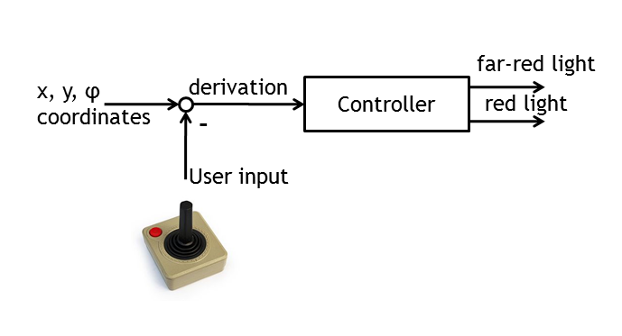
In order to safely guide E. lemming towards any desired target, a controller algorithm had to be developed. The inputs were defined to be as the current direction followed by the E. lemming, the reference direction, set by the user and the time point of the simulation. The outputs were Boolean values for red and far-red light pulses, to be applied at every time point of the simulation. The controller function was executed with the same frequency as images are made in the microscope. | In order to safely guide E. lemming towards any desired target, a controller algorithm had to be developed. The inputs were defined to be as the current direction followed by the E. lemming, the reference direction, set by the user and the time point of the simulation. The outputs were Boolean values for red and far-red light pulses, to be applied at every time point of the simulation. The controller function was executed with the same frequency as images are made in the microscope. | ||
| Line 32: | Line 37: | ||
* A controller which would set the red light and far-red light outputs independent of the current direction of the E. lemming will reach Γ≈1 for T>>1. | * A controller which would set the red light and far-red light outputs independent of the current direction of the E. lemming will reach Γ≈1 for T>>1. | ||
| - | The controllers of all | + | The controllers of all participants of the competition were run until the cost function Γ reached approximately a steady state. The participant with the lowest long-time value of his/her cost function obtained the prize from Jörg. The results are summarized in the following section. |
== Implemented Controllers == | == Implemented Controllers == | ||
In the following we will list all controllers we implemented ordered increasing by the long-time value of the cost function they achieved. All controllers are nevertheless available in the Lemming Toolbox. | In the following we will list all controllers we implemented ordered increasing by the long-time value of the cost function they achieved. All controllers are nevertheless available in the Lemming Toolbox. | ||
| - | |||
=== Threshold Optimized Controller (Winner of the Control Design Competition) === | === Threshold Optimized Controller (Winner of the Control Design Competition) === | ||
'''Cost function value of Γ=0.7703. Implemented by Simona Constantinescu.'''<br> | '''Cost function value of Γ=0.7703. Implemented by Simona Constantinescu.'''<br> | ||
| - | [[Image:SimonaWinner.png|thumb|400px]] | + | [[Image:SimonaWinner.png|thumb|400px|Sketch of the idea of the competition, '''after the competition''']] |
[[Image:ETH_igem_controller_threshold.png|thumb|400px|'''Sample path under the Threshold Optimized Controller'''. The black lines represent the reference rectangle around which the E. lemming was forced to travel. The blue thick curve represents the actual path of the E. lemming.]] | [[Image:ETH_igem_controller_threshold.png|thumb|400px|'''Sample path under the Threshold Optimized Controller'''. The black lines represent the reference rectangle around which the E. lemming was forced to travel. The blue thick curve represents the actual path of the E. lemming.]] | ||
| - | In approaching the | + | In approaching the controller competition challenge and obtaining the bottle of highly expensive wine promised by Jörg, my strategy was the following: |
| - | * develop a simple and efficient control algorithm, based on the intuitive idea of keeping the current direction if the difference between it and the reference direction is within well - chosen error bounds (i.e. apply red light) and change the current direction otherwise (''i.e'' apply far-red light). | + | * develop a simple and efficient control algorithm, based on the intuitive idea of keeping the current direction if the difference between it and the reference direction is within well - chosen error bounds (''i.e.'' apply red light) and change the current direction otherwise (''i.e'' apply far-red light). |
| - | * use the simple algorithm as a reference and compare the implementation of the other, more complicated ideas, with | + | * use the previously described simple algorithm as a reference and compare the implementation of the other, more complicated ideas, with this benchmark. |
| - | The particular features of our system under study made it very difficult to theoretically address all the challenges of nonlinearity, delay and, most important, stochasticity. A basic probability principle says that the efficiency of any deterministic strategy in handling a random process increases with the sample size. Asymptotically, nice theories can be used to defend against randomness and even reduce it to single point estimates. On the contrary, when analyzing very small sample sizes, stochasticity plays a crucial role and, most often, complex deterministic strategies have little or no effect in controlling the random process. In our case, the sample size was always 1, as we had to decide, at every time point, what Boolean values | + | The particular features of our system under study made it very difficult to theoretically address all the challenges of nonlinearity, delay and, most important, stochasticity. A basic probability principle says that the efficiency of any deterministic strategy in handling a random process increases with the sample size. Asymptotically, nice theories can be used to defend against randomness and even reduce it to single point estimates. On the contrary, when analyzing very small sample sizes, stochasticity plays a crucial role and, most often, complex deterministic strategies have little or no effect in controlling the random process. In our case, the sample size was always 1, as we had to decide, at every time point, what Boolean values red light and far red light should take. |
| - | As a first test, The Threshold Optimized Controller is checking whether the actual direction of the E. lemming is between 0 and 2π. Since Gaussian white noise is added to the received angle at every time point of the simulation, in some of the cases, the value of the angle might become negative or might exceed 2π | + | As a first test, The Threshold Optimized Controller is checking whether the actual direction of the E. lemming is between 0 and 2π. Since Gaussian white noise is added to the received angle at every time point of the simulation, in some of the cases, the value of the angle might become negative or might exceed 2π. If this happens, the controller sets the negative values back to 0 and the large ones back to 2π, as a noise - suppressing measure. |
| - | Next, two error bounds are defined, one for the case in which both angles are on the same side of the zero axis of the unit trigonometric circle ( | + | Next, two error bounds are defined, one for the case in which both angles are on the same side of the zero axis of the unit trigonometric circle (threshold1 = 1.5 rad) and another one for the case in which the angles are on different sides (threshold2 = 4.7 rad). This corresponds to an approximately π acceptance region or to approximately 50% of the 2π possible angles values on the unit circle. If the difference between the reference and the current direction, modulo 2π, is within these error bounds, the current direction is kept. Otherwise, a new direction is sampled. |
The other algorithms I implemented were: | The other algorithms I implemented were: | ||
* Storing the angle values and taking more complex decisions given the current and the previous directions. This strategy came at the cost of being inefficient before the sample size was large enough. Furthermore, the reference direction of the E. lemming was also changing, so the sample size had to be reset at 0, maybe too soon after reaching a large - enough size. Before testing the algorithm, it was debatable whether the benefit of reaching a large - enough size and acting in accordance to the defined strategy could exceed the cost of losing the objectivity of treating each sample independently. | * Storing the angle values and taking more complex decisions given the current and the previous directions. This strategy came at the cost of being inefficient before the sample size was large enough. Furthermore, the reference direction of the E. lemming was also changing, so the sample size had to be reset at 0, maybe too soon after reaching a large - enough size. Before testing the algorithm, it was debatable whether the benefit of reaching a large - enough size and acting in accordance to the defined strategy could exceed the cost of losing the objectivity of treating each sample independently. | ||
| - | * Fighting the microscope/image processing delay, by keeping the angle fixed and changing it only once every 0.9 seconds. This strategy came at the cost of keeping the same angle (maybe wrong) for 0.9 seconds, which is equivalent to 3 pulses. Before testing, it was also unclear whether the benefit of obtaining the real angle, without delay, would exceed the cost of not changing the angle every time the | + | * Fighting the microscope/image processing delay, by keeping the angle fixed and changing it only once every 0.9 seconds. This strategy came at the cost of keeping the same angle (maybe wrong) for 0.9 seconds, which is equivalent to 3 pulses. Before testing, it was also unclear whether the benefit of obtaining the real angle, without delay, would exceed the cost of not changing the angle every time the chance was given. |
As the system was subject to strong stochasticity, the benefits of none of the above strategies exceeded their costs, as compared to the Threshold Optimized Controller. Therefore, among all my tries, the minimal objective function value was obtained for the Threshold Optimized Controller. | As the system was subject to strong stochasticity, the benefits of none of the above strategies exceeded their costs, as compared to the Threshold Optimized Controller. Therefore, among all my tries, the minimal objective function value was obtained for the Threshold Optimized Controller. | ||
Latest revision as of 01:35, 16 November 2010
Controller
Yellow dot: the currently selected E. lemming. Yellow cone: the current swimming direction of E. lemming. Red arrow: the reference direction set by the controller. Bright red background: far-red light (inducing tumbling). Dark red environment: red light (inducing directed movement). Gray environment: both red and far-red light absent.
Note the small rectangle in the upper right corner of the image, along whose edges the E. lemming is forced to swim. As observed by the end of the simulation, the controller algorithm efficiently guides the E. lemming on the desired route.
Introduction
In order to safely guide E. lemming towards any desired target, a controller algorithm had to be developed. The inputs were defined to be as the current direction followed by the E. lemming, the reference direction, set by the user and the time point of the simulation. The outputs were Boolean values for red and far-red light pulses, to be applied at every time point of the simulation. The controller function was executed with the same frequency as images are made in the microscope.
The following properties of our network, consisting of both in silico and in vivo sub-parts, are making our task intractable for most theoretical controller design strategies:
- The chemotaxis network is highly nonlinear;
- Tumbling occurs stochastically;
- The angular change during tumbling is not predictable, neither the direction nor its absolute value;
- During directed movement periods, the angle is also changing stochastically (although not as much as during tumbling);
- Microscope, cell detection and tracking, and the approximation of the current angle of the E. lemming sum up to a time delay of approximately one second.
- The approximated angle is highly noisy.
As far as we are aware of, no theoretical controller design algorithm exists that can tackle all these challenges. To nevertheless develop several implementations which afterward can be compared in terms of performance, we decided to start a controller design competition between the team members.
In the following we first present the rules for the competition, which also include a measure for the performance of a controller, and afterward the different approaches developed by our team members together with their evaluation.
Controller Design Competition
The goal of the competition was to develop an implementation of a controller which performs best in forcing the E. lemming in swimming to a desired direction. Our instructor Jörg Stelling agreed, more or less voluntarily, to donate a bottle of highly expensive wine as a prize for the winner of the competition.
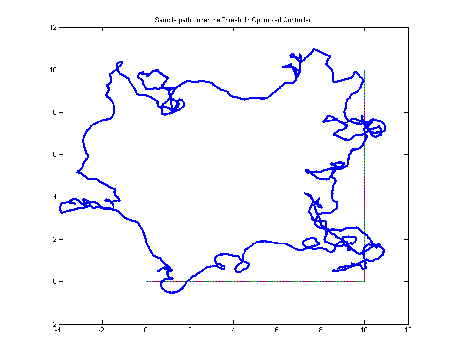
For the competition every participant had to force his or her E. lemming model to swim clockwise around a 1083×825μm large rectangle (approximately the size of 10 microscope images stringed together in each direction). Therefore, the reference direction send to the controller was set parallel to the axis of the coordinate system, and towards the next corner of the rectangle. Always when the Euclidean distance between the virtual E. lemming and the active corner was falling below 90μm (approximately the size of one microscope image), the next corner was activated.The current direction of the E. lemming obtained from the model was delayed for 0.9s and white noise was added, in order to simulate the conditions mentioned above. The controller algorithm was called every 0.3s and could either activate or deactivate the red and the far-red light. All other details for the construction of the controllers were left open.
For the evaluation of the controllers we defined the cost function Γ as following:
with T the evaluation time, φis the direction of the E. lemming, φsh the reference direction. The value of the cost function is always ∈[0,2] and can be interpreted as following:
- If Γ=0, the E. lemming would always swim exactly in the reference direction.
- If Γ=2, the E. lemming would always swim exactly opposite to the reference direction.
- A controller which would set the red light and far-red light outputs independent of the current direction of the E. lemming will reach Γ≈1 for T>>1.
The controllers of all participants of the competition were run until the cost function Γ reached approximately a steady state. The participant with the lowest long-time value of his/her cost function obtained the prize from Jörg. The results are summarized in the following section.
Implemented Controllers
In the following we will list all controllers we implemented ordered increasing by the long-time value of the cost function they achieved. All controllers are nevertheless available in the Lemming Toolbox.
Threshold Optimized Controller (Winner of the Control Design Competition)
Cost function value of Γ=0.7703. Implemented by Simona Constantinescu.
In approaching the controller competition challenge and obtaining the bottle of highly expensive wine promised by Jörg, my strategy was the following:
- develop a simple and efficient control algorithm, based on the intuitive idea of keeping the current direction if the difference between it and the reference direction is within well - chosen error bounds (i.e. apply red light) and change the current direction otherwise (i.e apply far-red light).
- use the previously described simple algorithm as a reference and compare the implementation of the other, more complicated ideas, with this benchmark.
The particular features of our system under study made it very difficult to theoretically address all the challenges of nonlinearity, delay and, most important, stochasticity. A basic probability principle says that the efficiency of any deterministic strategy in handling a random process increases with the sample size. Asymptotically, nice theories can be used to defend against randomness and even reduce it to single point estimates. On the contrary, when analyzing very small sample sizes, stochasticity plays a crucial role and, most often, complex deterministic strategies have little or no effect in controlling the random process. In our case, the sample size was always 1, as we had to decide, at every time point, what Boolean values red light and far red light should take.
As a first test, The Threshold Optimized Controller is checking whether the actual direction of the E. lemming is between 0 and 2π. Since Gaussian white noise is added to the received angle at every time point of the simulation, in some of the cases, the value of the angle might become negative or might exceed 2π. If this happens, the controller sets the negative values back to 0 and the large ones back to 2π, as a noise - suppressing measure.
Next, two error bounds are defined, one for the case in which both angles are on the same side of the zero axis of the unit trigonometric circle (threshold1 = 1.5 rad) and another one for the case in which the angles are on different sides (threshold2 = 4.7 rad). This corresponds to an approximately π acceptance region or to approximately 50% of the 2π possible angles values on the unit circle. If the difference between the reference and the current direction, modulo 2π, is within these error bounds, the current direction is kept. Otherwise, a new direction is sampled.
The other algorithms I implemented were:
- Storing the angle values and taking more complex decisions given the current and the previous directions. This strategy came at the cost of being inefficient before the sample size was large enough. Furthermore, the reference direction of the E. lemming was also changing, so the sample size had to be reset at 0, maybe too soon after reaching a large - enough size. Before testing the algorithm, it was debatable whether the benefit of reaching a large - enough size and acting in accordance to the defined strategy could exceed the cost of losing the objectivity of treating each sample independently.
- Fighting the microscope/image processing delay, by keeping the angle fixed and changing it only once every 0.9 seconds. This strategy came at the cost of keeping the same angle (maybe wrong) for 0.9 seconds, which is equivalent to 3 pulses. Before testing, it was also unclear whether the benefit of obtaining the real angle, without delay, would exceed the cost of not changing the angle every time the chance was given.
As the system was subject to strong stochasticity, the benefits of none of the above strategies exceeded their costs, as compared to the Threshold Optimized Controller. Therefore, among all my tries, the minimal objective function value was obtained for the Threshold Optimized Controller.
Hysteresis based Sliding Mode Controller
Cost function value of Γ=0.7727. Implemented by Moritz Lang.
|φis-φsh|mod 2π<π/2. However, this decrease can be small for larger differences in this set and especially near the destination a direction of the E. lemming only narrowly fulfilling this condition will soon get invalid due to the movement of the E. lemming nearly tangential to the reference direction. Furthermore, due to the slight changes in direction during swimming and the measurement error when determining the direction of the E. lemming, it can happen that, when the angle between the reference direction and the actual direction is near to π, the direction of the E. lemming "enters" and "leaves" this set very rapidly. A simple algorithm like "red light when the difference of the directions is smaller than π, otherwise far-red light" could then lead to rapid switching between the diodes, an effect not desirable in an experimental setup.
I thus decided to define two sets, Son={φis∈[0,2π):|φis-φsh|mod 2π<π/2} and Soff={φis∈[0,2π):|φis-φsh|mod 2π<π/3}. Furthermore the controller has two states, ζon and ζoff, and the state of the controller is maintained between evaluations of the controller algorithm.
When the controller is in state ζoff, it tests whether φis is in Soff or not. If the condition is fulfilled, a 2.4s (≈4 evaluations) red light pulse is send and the state is set to Son.
When the controller is in state ζon, it tests whether φis is in Son or not. If the condition is not fulfilled, a 2.1s (≈3 evaluations) far-red light pulse is send and the state is set to Soff.
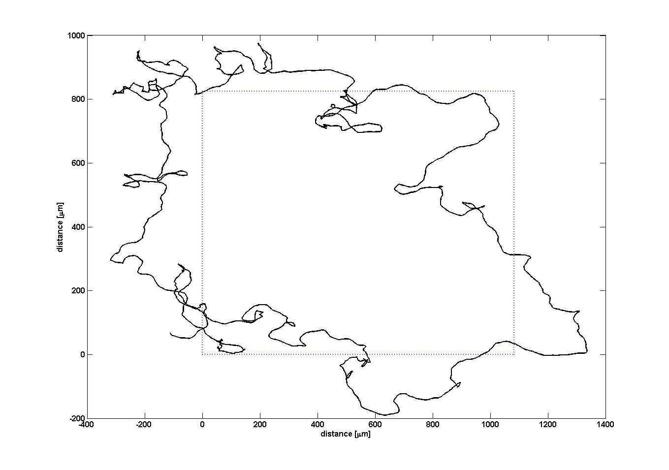
Our evaluations showed that this controller forces the E. lemming successful around the rectangle (see Figure on the right), while minimizing both light pulses.
Noise Refusing Subspace of Trust Controller
Cost function value of Γ=0.8089. Implemented by Christoph Hold.
The controller is a graduated response to the derivation of angles φder=|φset - φis| that takes advantage of an additional input signal. As there is two input binary signals this gives 4 possible input combinations:
| Input | Output | |
| red light | far red light | bias |
| 0 | 0 | as before |
| 1 | 0 | high |
| 0 | 1 | low |
| 1 | 1 | medium |
Additionally it is coupled with a noise suppression.
1. If the derivation of angle φder< αnarrow is small then by red light emission the bias is shifted as high as possible in order to keep the bacterium on the right track.
2. If the derivation of angle φder< αwide is acceptable, a compromise between going further that direction and tumbling is achieved by the usage of both red and far red light.
3. If the derivation of angle φder> αwide tumbling is initiated by far red light.
The angles of rules 1 and 2 are so chosen that the mean change in angle through tumbling will result in the optimal direction. A further element of the controller tries to distinguish between angle derivation due to the noisy angle signal and real tumbles and applies the last decision of rules 1 and 2 in order to prevent a wrong way induced by error.
Four Zones of Preference Controller
Cost function value of Γ=0.8196. Implemented by George Rosenberger.
A core problem of the very simple "red light when the difference of the directions is smaller than π, otherwise far-red light" algorithm is, that the edge between red and far-red light is very sharp. Therefore, the controller often changes between these two states and because of the time delay of the microscope and image processing, prediction of best light pulse tends to be inaccurate at this threshold.
The core concept of this controller is to extend the very basic algorithm in a way, that the edge between red and far-red light is avoided, e.g. it should be leaped. This is achieved by creating a dark area of 2 * 15° between red and far-red thresholds, in which no light pulse is being sent at all. Next to the far-red light zone, the repeating times are increased in an order to possibly leap the dark area and go to a different angle, better (or worse) than the dark area.
Majority Vote Proportional - Second Derivative Threshold Controller
Cost function value of Γ=0.8379. Implemented by Thanuja Ambegoda.
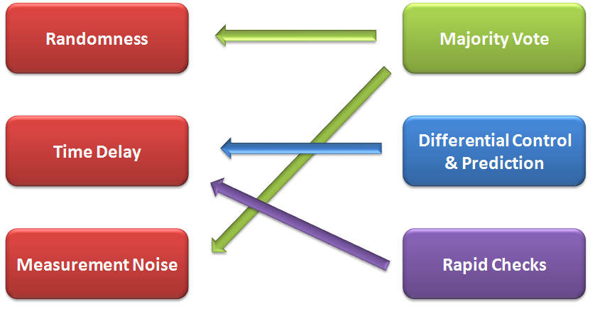
What the controller needs to do boils down to the following: When the cell is going in the wrong direction, make it tumble until each heads towards the right direction. When it is heading towards the right direction, try to keep it in the swimming mode. But, the task is slightly complicated by the presence of the following 'obstacles':
- Randomness of the motion – the direction changes slightly (randomly) when swimming and it changes rapidly with larger angles when tumbling.
- Noise in measurement: the error we measure is not the exact error
- Time delay of measurement – the measurement of error is not the current error. It's around 1 second before now.
In the absence of the above three, the controller would have been trivial. This particular controller tries to minimize the effects of these by deploying an algorithm that incorporates the following features:
- Majority voting based on historical error - This is a way of fighting noise. When deciding if error correction needs to be deployed (force tumbling), the controller not only looks at the current error. But also, it tries to deduce if there is a real error by looking at the reported error of a few previous samples. Majority voting is also used with differential error prediction (described later) at different levels of control inside the algorithm.
- Rapid Checks - A slight variation to the above majority voting, used to detect larger errors, quickly. A slightly higher margin of error is allowed with a lower number of previous samples, when there is a need to detect a larger error quickly. A similar setting can be used with a lower threshold to detect quick returns to the correct direction
- Error prediction based on differential control - This is used to minimize the effects of the time delay of measurements. Differential error is considered in conjunction with the reported error evaluated using the majority voting scheme.
 "
"


