Team:Heidelberg/Modeling/descriptions
From 2010.igem.org
(→Parameterization Concept) |
(→Simulation and experimental verification) |
||
| (138 intermediate revisions not shown) | |||
| Line 1: | Line 1: | ||
| - | {{:Team:Heidelberg/ | + | {{:Team:Heidelberg/Single}} |
{{:Team:Heidelberg/tables|normal=FFF|highlight=ddd}} | {{:Team:Heidelberg/tables|normal=FFF|highlight=ddd}} | ||
| - | |||
| - | =Modeling | + | {{:Team:Heidelberg/Single_Pagetop|modelset}} |
| + | {{:Team:Heidelberg/Side_Top}} | ||
| + | |||
| + | __TOC__ | ||
| + | |||
| + | {{:Team:Heidelberg/Side_Bottom}} | ||
| + | |||
| + | =miBEAT:= | ||
| + | |||
| + | miBEAT ('''mi'''RNA '''B'''inding site '''E'''ngineering and '''A'''ssembly '''T'''ool) is a graphical user interface that has as its back-end a compilation of multiple individual models and scripts which interact with each other to generate constructs. | ||
| + | |||
| + | ==miRockdown== | ||
| + | |||
| + | miRNA binding sites of varying binding efficiencies can be used to manipulate levels of proteins in a cell. Several tools can predict mRNA knockdown, but our approach aims for the final objective: protein levels (specially interesting for medical applications like gene therapy). This approach, offers a more complete result than the computational tools available, that focus on mRNA levels. | ||
| + | |||
| + | ===How to use miRockdown=== | ||
| + | The modeling project was planned in a way such that the model predictions would be available online in the form of a GUI. We made it in the most user-friendly way we could think of: The user only needs to input the desired knockdown percentage (kd%) and choose an sh/miRNA sequence, to get a binding site to satisfy their needs.<br> | ||
| + | <br> | ||
| + | <center>[[Image:Modscheme.png|400px]]<br><br> | ||
| + | <div style="font-size:0.95em;" width="400"><b>Overview of the miRockdown script flow.</b><br> | ||
| + | The knockdown percentage (kd%) input invokes the selection of the appropriate experimental BS or theoretical binding site parameters. The miRNA sequence starts the generation of BS sequences. Subsequently, these BS sequences are characterized by a modified TargetScan algorithm and finally the parameters of the theoretical BS are compared with the parameters of the generated BSs and the closest of the generated BSs is given as output.</div></center> | ||
| + | <br><br> | ||
| + | The results of both of our models and the experimentally verified binding sites are integrated in [https://2010.igem.org/Team:Heidelberg/Modeling/miRockdown miRockdown] on [https://2010.igem.org/Team:Heidelberg/Modeling/miGUI miBEAT]. | ||
| + | For every binding site request of a user he receives the results of the three different approaches. Thus the user can always choose which of the three differently generated binding sites they want to use. | ||
| + | The binding site with the closest experimentally observed knockdown percentage is displayed, together with its properties and oligos ready to clone into the [https://2010.igem.org/Team:Heidelberg/Project/miRNA_Kit miTuner]-construct.<br> | ||
| + | The binding sites generated using the models are useful when the user wants to use their own sh/miRNA or when there are not close enough experimentally verified binding sites.<br> | ||
| + | A script integrated into miRockdown will correlate the desired kd% with a database for every model. This database consists of a set of binding site parameter objects spanning the complete range of parameters. Additionally, the database contains the models' knockdown percentage calculated for the whole set of objects.<br> | ||
| + | With the user-chosen sh/miRNA sequence as input, a binding site generator script is invoked, which created more than 2000 different BS on-the-fly by varying the seed-type, 3'pairing, AU content and bulge size. The 3'pairing and the AU content score of the generated BS are characterized by a modified version of the TargetScan Algorithm {{HDref|Rodriguez et al., 2007}}. The input and output functions of the algorithm were adapted for miRockdown, so that no files have to be generated.<br> | ||
| + | Now that the generated binding sites are completely characterized, they are compared with the parameters of the suitable model BS. The generated BS that fits best the parameters of the suitable model BS is selected as the output BS of miRockdown. | ||
| + | |||
| + | <html> | ||
| + | <div class="backtop"> | ||
| + | <a href="#top">↑</a> | ||
| + | </div> | ||
| + | </html> | ||
| + | |||
| + | ==miBSdesigner== | ||
| + | Having a binding site designer was crucial to complete the computational approach to our project: miBSdesigner is an easy-to-use application to create in silico binding sites for any given miRNA. Using our device, the user will be able to generate binding sites with several different properties. | ||
| + | |||
| + | ===Input=== | ||
| + | The user has to input a name for the miRNA to name the primers. The miRNA sequence must be 22 nucleotides long and has to be input in direction 5’ to 3’ (both DNA and RNA sequences are admitted and any extra characters will be removed from the sequence). The user can also enter a spacer inert sequence if he needs to place the binding site further along in the 3’UTR region (it is recommended that the binding site is at least 15 nucleotides away from the stop codon). | ||
| + | Initially the user can choose between a perfect binding site (matching the 22 nucleotides), or an almost perfect binding site (matching all of the nucleotides, but leaving a 4-nucleotide bulge between 9 and 12. | ||
| + | Apart from these two options, the user can further modify the binding site to meet their individual requirements. | ||
| + | |||
| + | ===Seed Types=== | ||
| + | <center>[[Image:Final_sequences_miRNAseeds.png|800px]]</center> | ||
| + | |||
| + | Figure 1: Interactions between two miRNAs and their binding sites with different types of seeds. | ||
| + | |||
| + | |||
| + | In miBS designer, the user can choose between several types of seed for their binding site (list ordered by increasing efficacy): | ||
| + | |||
| + | - 6mer (abundance 21.5%): only the nucleotides 2-7 of the miRNA match with the mRNA. | ||
| + | |||
| + | - 7merA1 (abundance 15.1%): the nucleotides 2-7 match with the mRNA, and there is an adenine in position 1. | ||
| + | |||
| + | - 7merm8 (abundance 25%): the nucleotides 2-8 match with the mRNA. | ||
| + | |||
| + | - 8mer (abundance 19.8%): the nucleotides 2-8 match with the mRNA and there is an adenine in position 1. | ||
| + | |||
| + | - Apart from any of these options, the user can decide to create a customized seed with one mismatch included. By inputting a number (between 2-7) in the Customized mismatch position textbox | ||
| + | |||
| + | The percentages of abundance are calculated among conserved mammalian sites for a highly conserved miRNA {{HDref|Bartel (2009)}}. | ||
| + | |||
| + | ===Supplementary Region=== | ||
| + | In miBS designer, the user can choose among several types of supplementary regions, starting with 3 matching nucleotides (14-16), increasing sequentially until 8 (13-20), and then total matching (from 13-22, leaving a bulge){{HDref|Grimson A et al(2007)}}. | ||
| + | In case the user needs some other specific supplementary region, he can customize the sequence by inputting the desired matching nucleotides (in numbers from 9 to 22, separated by commas). | ||
| + | |||
| + | ===AU Content=== | ||
| + | In order to allow the user to improve the efficiency of their binding sites, miBS designer offers options to increase the AU content by adding adenine or uracil to positions around the matches (specifically in -1, 0, 1, 8, 9 and 10). The function is designed so that it varies the AU content without introducing new pairings. | ||
| + | |||
| + | ===Sticky Ends=== | ||
| + | To facilitate the task of introducing the binding site into a plasmid, the user can add sequences to both ends of the binding site. Initially, the user can choose among the [http://openwetware.org/wiki/The_BioBricks_Foundation:RFC#BBF_RFC_12:_Draft_BioBrick.E2.84.A2_BB-2_standard_for_biological_parts RFC-12 standard for biobricks BB2], the XmaI/XhoI restriction enzymes used in our [https://2010.igem.org/Team:Heidelberg/Project/miRNA_Kit miTuner]-construct, or some custom sequences input by the user. In the last case, the output sequences will not be directly ready for cloning: the user has to either digest the construction prior to ligation, or to process the primers before ordering them to remove the extra nucleotides and create the overhangs. | ||
| + | |||
| + | ===Output=== | ||
| + | miBS designer generates the primer needed to integrate the binding site desired into a plasmid, alongside with the primer for the complementary strand. It will also produce specific names for the two primers. | ||
| + | |||
| + | ==mUTING== | ||
| + | It is a tool developed to generate binding sites for miRNAs that could be used for tissue targeting based on both on- as well as off-targeting strategy. It takes as input the target and off-target tissues as well as the desired targeting strategy. User can also specify a threshold for difference in the level of relative expression (within a tissue) of miRNAs between target and off-target tissue. The program searches through a database of expression levels to give out a list of possible miRNAs which could be used. Out of these, the desired miRNA can be selected for which the final output is generated in the form of sense and anti-sense oligomers with overhangs that could be used to put binding sites in tandem or into a vector. | ||
| + | |||
| + | ===Input=== | ||
| + | |||
| + | The input for the tool is rather simple and consists of five fields. | ||
| + | |||
| + | '''Organism''' – The tool lets you choose between Human, Rat and Mouse as the source organism. | ||
| + | |||
| + | '''Target''' – From a list of tissues, the target (tissue where gene has to be expressed) can be selected. | ||
| + | |||
| + | '''Off-target''' – A list from which multiple off-targets can be selected is available. Here, the tissues from which gene expression has to be excluded can be included. | ||
| + | |||
| + | '''Targeting''' – This options lets you select the targeting strategy you want to employ. | ||
| + | |||
| + | '''Threshold''' – The threshold for difference in the level of relative expression of miRNA in the target and off-target tissue can be set here. The default value is 0.001. | ||
| + | |||
| + | ===Data=== | ||
| + | The expression data and sequence data that the tool makes use of was recruited from preexisting data sources. | ||
| + | |||
| + | '''Sequences''' – mature miRNA sequences were obtained from mirBase Sequence Database Release 16 {{HDref|Griffiths-Jones S. et al.(2008)}}. | ||
| + | |||
| + | '''Expression profiles''' - miRNA expression profiles were collected from a previously published resource of 172 human, 64 mouse and 16 rat small RNA libraries extracted from major organs and cell types {{HDref|Landgraf et al.(2007)}}. The expression values in the data represent the number of cloned mature microRNAs that were sequenced in each library and reported as clone counts. The counts are normalized by the total number of microRNAs that were cloned in each library. These values are then used to calculate the difference in relative miRNA levels for differential expression of the construct. | ||
| + | |||
| + | ===Processing=== | ||
| + | The processing of the data has been done by script written in PERL. After submitting the primary inputs, mentioned above, the tool gives the user a choice of different miRNAs that fulfill the criterion set in the input. These are displayed along with the miRNA expression values in the target (in case of off-targeting) or in the off-targets (in case of on-targeting). The expression values in the off-targets and target in the respective cases are required to be zero. Based on these values, the user can select the most suitable miRNA for their construct. | ||
| + | |||
| + | ===Output=== | ||
| + | The final output is the binding site for the miRNA selected by the user. It consists of the sense strand and the anti-sense strand that would code the binding site. These are flanked by a spacer sequence that could be used for putting binding sites in tandem and for introducing cloning sites. | ||
| + | |||
| + | =Modeling= | ||
| + | |||
| + | The Neural Network and the Fuzzy Logic Model explained here are the basis of the [https://2010.igem.org/Team:Heidelberg/Modeling/miRockdown miRockdown] tool. The results of the optimized models are integrated as a database and enable the [https://2010.igem.org/Team:Heidelberg/Modeling/trainingset#miRockdown miRockdown] output of binding sites, to have confidently predicted protein knockdown efficiency. | ||
| + | |||
==Parameterization Concept== | ==Parameterization Concept== | ||
| - | One of the hardest tasks in the development of our models was to come up with good strategy to generate input parameters from the raw data. In our case, the raw data is the binding site sequence and the corresponding sh/miRNA-sequence. The final parameterization concept unites a basic distinction between perfect, bulged (near-perfect) and endogenous miRNA like BS, with the advanced 3'-scoring and AU-content evaluation. The endogenous miRNA like BS parameter is further split into the three [Modeling# | + | One of the hardest tasks in the development of our models was to come up with good strategy to generate input parameters from the raw data. In our case, the raw data is the binding site sequence and the corresponding sh/miRNA-sequence. The final parameterization concept unites a basic distinction between perfect, bulged (near-perfect) and endogenous miRNA like BS, with the advanced 3'-scoring and AU-content evaluation. The endogenous miRNA like BS parameter is further split into the three [https://2010.igem.org/Team:Heidelberg/Modeling#miRNA_binding_site_features seed-types]. |
| + | The targetscan_scores_50-algorithm {{HDref|Rodriguez et al., 2007}} was used to characterize binding sites in respect to 3'-pairing and AU-content score. TargetScan aligns the miRNA with the mRNA sequence starting from a given seed-position in a way the highest possible 3'-score is reached. Binding from miRNA nucleotide 13-16 will add 1 to the score, pairings outside this region add 0.5. Offsets between bound miRNA and mRNA are also allowed, but will there is a penalty of 0.5 points for an offset higher than 2 nucleotides. The AU-content of 30 nucleotides upstream and downstream of the mRNA seed sequence is rated seed type dependent. The impact of the nucleotides decreases with the distance from the seed. The scoring system is based on a regressions applied to datasets from human, mouse, rat and dog mRNA knockdown {{HDref|Grimson et al., 2007}}. | ||
| + | |||
| + | Since all major prior modeling approaches used mRNA levels as training-set, our approach needs to will give a completely new insight into miRNA binding site functionality. | ||
| + | {| class="wikitable" | ||
| + | | [[Image:3primevsAU.png|thumb]] | ||
| + | | [[Image:ThreePrimevsbulgeSize.png|thumb]] | ||
| + | | [[Image:SeedTvsthreePScore.png|thumb]] | ||
| + | | [[Image:SeedTvsAUScore.png|thumb]] | ||
| + | |} | ||
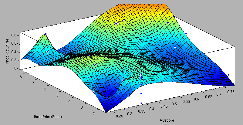
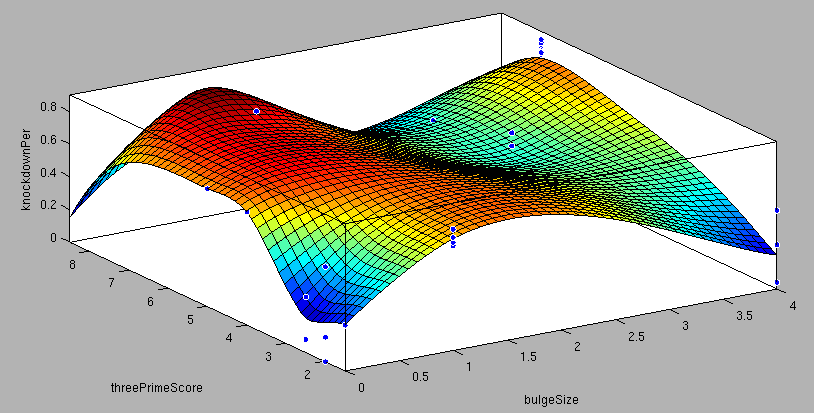
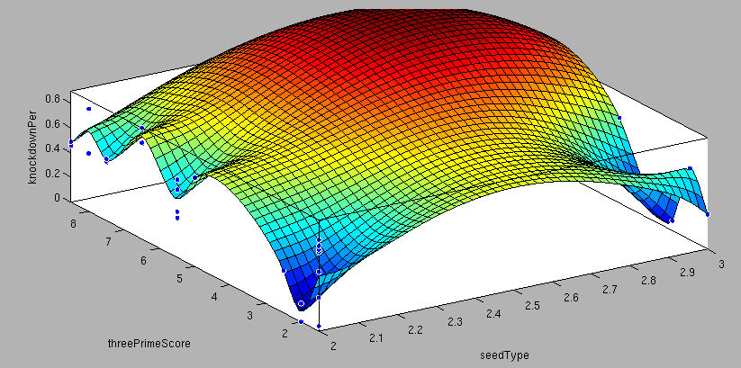
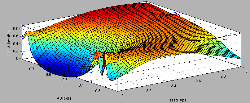
| + | <center>3'-pairing-Score vs AU-content-Score/ThreePrime vs BulgeSize/SeedType vs 3'pairing-Score/SeedType vs AU-score/ vs knockdown percentage of the training set data: <br> | ||
| + | These surface fits show the correlation of increasing 3' Binding Score and AU content Score with increasing knockdown-efficiency of the binding sites. Also the other parameters nicely correlate with our expectations.</center> | ||
| + | <br><br> | ||
| + | |||
| + | ==Neural Network Model== | ||
| + | |||
| + | ===Neural Network theory=== | ||
| + | Artificial Neural Network usually called (NN), is a computational model that is inspired by the biological nervous system. The network is composed of simple elements called artificial neurons that are interconnected and operate in parallel. In most cases the NN is an adaptive system that can change its structure depending on the internal or and external information that flows into the network during the learning process. The NN can be trained to perform a particular function by adjusting the values of the connection, called weights, between the artificial neurons. Neural Networks have been employed to perform complex functions in various fields, including pattern recognition, identification, classification, speech, vision, and control systems. | ||
| + | Mathematically there are three basic components that describes a single layer network: the synapses of the artificial neurons that are modeled as weights and that represent how strong is the connection between the input and an artificial neuron. An adder, that sum up all the the weighted inputs and finally an activation function, that controls the amplitude of the output of the single layer. Generally there are three type of activation function: threshold, sigmoid, piecewise linear function. For our model the sigmoid function has been used, it can range the output between 0 and 1 or between -1 and 1 {{HDref|Kröse et al, 1996}}.<br> | ||
| + | <center>[[Image:NeuralNetwork_HD2010_image2.png|400px]]<br> | ||
| + | Figure 2: representation of the mathematical model of a biological neuron.</center><br> | ||
| + | <br> | ||
| + | During the learning process, difference between the desired output (target) and the network output is minimised. This difference is usually called cost; the cost function is the measure of how far is the network output from the desired value. A common cost function is the mean-squared error and there are several algorithms that can be used to minimise this function. The following figure displays such a loop. | ||
| + | |||
| + | <center>[[Image:Neural_Network.png]]<br> | ||
| + | Figure 3: Training of a Neural Network.</center> | ||
| + | |||
| + | ===Model description=== | ||
| + | |||
| + | ====Input/target pairs==== | ||
| + | The NN model has been created with the MATLAB NN-toolbox. The input/target pairs used to train the network comprise experimental and literature data {{HDref|Bartel et al., 2007}}. The experimental data were obtained by measuring via luciferase assay the strength of knockdown due to the interaction between the shRNA and the binding site situated on the 3’UTR of luciferase gene ([https://2010.igem.org/Team:Heidelberg/Project/miRNA_Kit miTuner]). Nearly 30 different rational designed binding sites were tested and the respective knockdown strength calculated.<br> | ||
| + | Each input was represented by a four elements vector. Each element corresponded to a score value related to a specific feature of the binding site (as mentioned in the previous paragraph "Parametrization concept"). The three features used to describe the binding site were: seed type, the 3’pairing contribution and the AU-content. The input/target pair represented the relationship between a particular binding site and the related percentage of knockdown. | ||
| + | Two Neural Network were trained. One was trained with a pool of 45 data coming from literature. The other one was trained with experimental data. The latter network comprised 4 inputs instead of 3. the fourth input represented the size of the bulge in base pairs. Afterwards both networks were used to predict percentages of knockdown given certain inputs. The predictions were then validated experimentally and compared among the different networks. | ||
| + | |||
| + | ====Characteristic of the Network==== | ||
| + | |||
| + | The neural network comprised two layers (multilayer feedforward Network). The first layer is connected with the input network and it comprised 15 artificial neurons. The second layer is connected to the first one and it produced the output. For the first and the second layer a sigmoid activation function and a linear activation function were used respectively. The algorithm used for minimizing the cost function (sum squared error) was Resilient Back Propagation (RPROP). RPROP has proven to be one of the best in terms of speed of convergence, moreover it can eliminate the harmful effect of sigmoid activation function used in the hidden layer.<br> | ||
| + | [[Image:viewnet.png|center]]<br> | ||
| + | <br> | ||
| + | Figure 3: schematic illustration of the network components. Hidden represent the first layer and it comprised 15 artificial neurons, while output is the second and last layer producing the output. The symbol “w” was the representation of the weights and “b” of the biases. | ||
| - | == | + | ===Results=== |
| - | {| border="1" class="wikitable | + | Two experiment batches were performed. The network trained only with data coming from literature was used to predict the outcome of the first experiment batch. In Table 1 the simulated and experimental percentage of knockdown are showed. It becomes clear by looking the results that the bulge size has indeed an effect on the knockdown percentage, in fact the network is able to simulate with high precision when the bulge size is on the range of 3 and 4 nt, but not when it becomes 1 or 0. It is important to underly here that the network was trained with literature values that did not take into consideration the bulge size as a key factor, TargetScan in fact, does not evaluate this binding site feature in the scoring process. The importance of the bulge size is also emphasized in the surface plot in the "Parametrization concept" .<br> |
| - | !align="right"| | + | <center> |
| + | {| border="1" class="wikitable sortable" cellpadding="6" style="border:solid 1px #AAAAAA; border-collapse:collapse; background-color:#F9F9F9; empty-cells:show; font-size:0.9em;" | ||
| + | !align="right"| 3' score !! AU-score !! bulge !! seed type !! bulge size !! number BS !! KD% experimental !! KD% simulated | ||
|- | |- | ||
| - | |align="right"| | + | |align="right"| 7.5 || 0.624 || 1 || 3 || 4 || 1 || 0.85 || 0.82 |
|- | |- | ||
| - | |align="right"| | + | |align="right"| 7.5 || 0.595 || 1 || 3 || 4 || 1 || 0.81 || 0.81 |
|- | |- | ||
| - | |align="right"| | + | |align="right"| 7.5 || 0.576 || 1 || 3 || 4 || 2 || 0.92 || 0.8 |
|- | |- | ||
| - | |align="right"| | + | |align="right"| 4 || 0.314 || 0 || 3 || 0 || 1 || 0.69 || 0.56 |
|- | |- | ||
| - | |align="right"| | + | |align="right"| 2.5 || 0.314 || 0 || 3 || 0 || 1 || 0.08 || 0.49 |
|- | |- | ||
| - | |align="right"| | + | |align="right"| 5 || 0.336 || 0 || 2 || 0 || 1 || 0.72 || 0.42 |
|- | |- | ||
| - | |align="right"| | + | |align="right"| 1.5 || 0.327 || 0 || 3 || 0 || 1 || 0.28 || 0.44 |
|- | |- | ||
| - | |align="right"| | + | |align="right"| 2 || 0.327 || 0 || 3 || 0 || 1 || 0.58 || 0.46 |
|- | |- | ||
| - | |align="right"| | + | |align="right"| 2.5 || 0.221 || 0 || 2 || 0 || 1 || 0.34 || 0.28 |
|- | |- | ||
| - | |align="right"| | + | |align="right"| 7.5 || 0.597 || 1 || 3 || 4 || 1 || 0.82 || 0.81 |
|- | |- | ||
| - | |align="right"| | + | |align="right"| 7.5 || 0.603 || 1 || 3 || 4 || 1 || 0.83 || 0.81 |
|- | |- | ||
| - | |align="right"| | + | |align="right"| 7.5 || 0.624 || 1 || 3 || 4 || 1 || 0.77 || 0.82 |
|- | |- | ||
| - | |align="right"| | + | |align="right"| 7.5 || 0.6 || 1 || 3 || 4 || 1 || 0.76 || 0.81 |
|- | |- | ||
| - | |align="right"| | + | |align="right"| 7.5 || 0.603 || 1 || 3 || 4 || 1 || 0.82 || 0.81 |
|- | |- | ||
| - | |align="right"| | + | |align="right"| 5.5 || 0.799 || 1 || 2 || style="background-color:#cacaca;" | 3 || 1 || style="background-color:#cacaca;" | 0.59 || style="background-color:#cacaca;" | 0.63 |
|- | |- | ||
| - | |align="right"| | + | |align="right"| 5.5 || 0.749 || 1 || 2 || 3 || 1 || 0.345 || 0.61 |
|- | |- | ||
| - | |align="right"| | + | |align="right"| 6.5 || 0.799 || 1 || 2 || style="background-color:#cacaca;" | 1 || 1 || style="background-color:#cacaca;" | 0.9 || style="background-color:#cacaca;" | 0.67 |
|- | |- | ||
| - | |align="right"| | + | |align="right"| 6.5 || 0.773 || 1 || 2 || 1 || 1 || 0.775 || 0.67 |
|- | |- | ||
| - | |align="right"| | + | |align="right"| 1.5 || 0.38 || 1 || 2 || style="background-color:#cacaca;" | 1 || 1 || style="background-color:#cacaca;" | 0.68 || style="background-color:#cacaca;" | 0.27 |
|- | |- | ||
| - | |align="right"| | + | |align="right"| 1.5 || 0.38 || 1 || 2 || style="background-color:#cacaca;" | 4 || 1 || style="background-color:#cacaca;" | 0.21 || style="background-color:#cacaca;" | 0.27 |
|- | |- | ||
| - | |||
| - | |||
| - | |||
| - | |||
| - | |||
| - | |||
| - | |||
| - | |||
| - | |||
| - | |||
| - | |||
| - | |||
| - | |||
| - | |||
| - | |||
| - | |||
| - | |||
| - | |||
| - | |||
| - | |||
| - | |||
| - | |||
| - | |||
| - | |||
| - | |||
| - | |||
| - | |||
| - | |||
| - | |||
| - | |||
| - | |||
| - | |||
| - | |||
| - | |||
| - | |||
| - | |||
| - | |||
| - | |||
| - | |||
| - | |||
| - | |||
| - | |||
| - | |||
| - | |||
| - | |||
| - | |||
| - | |||
| - | |||
| - | |||
| - | |||
| - | |||
| - | |||
| - | |||
| - | |||
| - | |||
| - | |||
| - | |||
| - | |||
| - | |||
| - | |||
| - | |||
| - | |||
| - | |||
| - | |||
| - | |||
| - | |||
| - | |||
| - | |||
| - | |||
| - | |||
| - | |||
| - | |||
| - | |||
| - | |||
| - | |||
| - | |||
| - | |||
| - | |||
| - | |||
| - | |||
| - | |||
| - | |||
| - | |||
| - | |||
| - | |||
|} | |} | ||
| + | Table 1: it shows the simulated data and the experimental results given the features of the binding site. The values in red, underline the discrepancy that occur between the two set of knockdown when the bulge size is the only feature changing. When the bulge size is not 1 the prediction are very precise and within the standard deviation of the experimental values (between 10-25%).<br></center> | ||
| + | <br> | ||
| + | |||
| + | ====Brief conclusion==== | ||
| + | The bulge size was identified as a very important parameter for knockdown efficiency. This led us to the conclusion of training another Neural Network only with our experimental data and encompassing the bulge size in the input vector. | ||
| + | |||
| + | <html> | ||
| + | <div class="backtop"> | ||
| + | <a href="#top">↑</a> | ||
| + | </div> | ||
| + | </html> | ||
| + | ====Simulation and experimental verification==== | ||
| + | <br> | ||
| + | [[Image:regression1.png|300px|left]][[Image:regression2.png|300px|right]] | ||
| + | <br> | ||
| + | <br> | ||
| + | <br> | ||
| + | <br> | ||
| + | <br> | ||
| + | <br> | ||
| + | <br> | ||
| + | <br> | ||
| + | |||
| + | ==Fuzzy Logic Model== | ||
| + | ===Why using a fuzzy inference system to model binding site efficiency?=== | ||
| + | |||
| + | To be able to evaluate the complex features of an shRNA or miRNA binding site and predict a resulting knockdown percentage of the protein we developed a fuzzy inference system (fis). The parameterized properties of the binding sites serve as input and will be processed into the knockdown percentage as the single output. Thus our fuzzy inference system is characterized as a multiple input, single output fuzzy inference system (MISO). | ||
| + | |||
| + | Fuzzy Logic is a rule-based approximate artificial reasoning method developed by Lotfi Zadeh in 1965. Its motivation is the observation that humans often think and communicate in a vague way, and yet can make precise decisions {{HDref|Nelles O (2000)}}. It has been widely used in engineering and Artificial Intelligence approaches such as Fuzzy Controllers and Fuzzy Expert Systems. Fuzzy Logic has also been used for the modeling of biological pathways {{HDref|Bosl et al (2007)}} and to analyze gene regulatory networks {{HDref|Laschov et al(2009)}}. Key advantages of Fuzzy logic-based approaches are (i) the ability to construct models based on prior knowledge of the system and experimental data and (ii) encode intermediate states for inputs and outputs, thus improving other logic-approaches that can only deal with ON/OFF states such as Boolean models {{HDref|Aldridge et al (2009)}} and (iii) simulations can be derived from both qualitative and quantitative data, both of which can be cast into the form of IF-THEN rules. Thus, FL constitutes a powerful approach for the understanding of heterogeneous datasets. | ||
| + | |||
| + | Fuzzy inference systems are based on membership functions (MF). MFs rate input parameters how much they satisfy a criterion on a scale from 0 to 1. There can be one, or multiple MFs per input parameter. Like different criteria applied to an input. The height of persons for example can be evaluated with one MF - how much the person satisfies being tall. On the other hand, there could be 3 MFs, one evaluating the membership to small people, the second to medium sized people and the third one to big people. Changing the shape of the MF gives the opportunity to have either functional dependencies, allowing intermediate states of the membership values, or simple ON/OFF states, where the membership value can be only 0 or 1. Thus different kinds of input parameters can be evaluated with a fuzzy inference system. For the simple height example model the age of the person could be taken as second input and evaluated by a MF that is 0 until the age of 18 and 1 for older persons. Thus the model could differentiate between young and grown-up persons. | ||
| + | |||
| + | Simple if-then rules can then be used to combine the input MF to an output MF. The satisfaction of a rule by an object (set of input parameters) is defined by the degree of membership of the object to the different MFs. The higher the satisfaction of the rule, the higher is the membership to the output MF. | ||
| + | The output MF can be a function like the input MF. This is the case in Mamdani method fuzzy inference systems {{HDref|Mamdani et al, (1975)}}. We are using a Sugeno method fuzzy inference system {{HDref|Sugeno(1985)}}, where the output MF is either a constant or a linear function depending on input parameters. The advantage of a Sugeno fuzzy inference system is, that it is computationally more efficient and easier to optimize or adapt due to the more simple output MF. Due to the non-intuitive combination of the 3'-pairing- and AU-content score, our fuzzy inference system needs to be optimized computationally. | ||
| + | |||
| + | ===Fuzzy Model Concepts=== | ||
| + | |||
| + | Our fuzzy inference system can deal with 3 different kinds of shRNA binding sites. Perfect, bulged and endogenous-like binding sites are treated separately, due to the differences in their biological mechanism, as discussed earlier [link to binding site properties]. | ||
| + | A perfect binding site is evaluated by a simple ON/OFF input MF evaluating the boolean input of | ||
| + | |||
| + | We came up with different concepts of what kind of input parameters to integrate into the fuzzy inference model and how to evaluate them. Therefore we parameterized the [https://2010.igem.org/Team:Heidelberg/Modeling/trainingset properties of a large set of binding sites] according to various different BS characteristics. | ||
| + | The targetscan_50_context_scores – Algorithm {{HDref|Rodriguez et al., 2007}} which evaluates binding sites in respect to 3'-pairing and AU-content gives out a score that seems appropriate to distinguish especially between endogenous miRNA like binding sites. A more detailed description on the concept of binding site parameterization can be found under [https://2010.igem.org/Team:Heidelberg/Modeling/trainingset Model Training Set]. | ||
| + | |||
| + | |||
| + | {| class="wikitable" | ||
| + | |||
| + | | [[Image:Nearperfect.png|thumb|Bulged binding sites concept: This model concept evaluates bulged- or "near-perfect" binding sites separately from conventional seed + 3'-pairing binding sites. Rule number 2 considers the bulge-size of the bulged binding site.]] | ||
| + | | [[Image:BulgeAU.png|thumb|Bulged binding sites (including AU-content-score) concept: This concept extends the bulged-BS concept with the addition of AU-content score evaluation. Therefore rule number 2 was modified accordingly.]] | ||
| + | |||
| + | | [[Image:LowthreePrime.png|thumb|Consider low 3' score concept: This model concept takes into consideration, that binding sites with a 3'-score under 3 did not show a significant change in knockdown efficiency compared to a control with only seed pairing {{HDref|Grimson et al., 2007}}. This is realized by rule number 6.]] | ||
| + | |||
| + | |} | ||
| + | |||
| + | <html> | ||
| + | <div class="backtop"> | ||
| + | <a href="#top">↑</a> | ||
| + | </div> | ||
| + | </html> | ||
| + | |||
| + | ===Fuzzy Model Optimization=== | ||
| + | |||
| + | The Fuzzy Logic Toolbox and Global Optimization Toolbox were linked via a script and the output membership functions, as well as the input membership function parameters were optimized. | ||
| + | |||
| + | ===Result=== | ||
| + | {| class="wikitable" | ||
| + | | [[Image:ModelFit.jpg|thumb|Regression of Fuzzy Logic Model resulst vs Experimental results: The Fuzzy Logic Model is able to predict experimental results.]] | ||
| + | | [[Image:AUvs3primeModel.png|thumb|Correlation of AU-content-Score and 3'-pairing Score with knockdown% in the optimized model]] | ||
| + | |} | ||
| + | |||
| + | |||
| + | |||
| + | |||
| + | [http://igem.bioquant.uni-heidelberg.de/igem_2010/FuzzyModelResults.html Click here, if you are interested in more recent model optimizations results!] | ||
| + | |||
| + | =Data Overview= | ||
| + | The data used for training the models can be accessed [https://2010.igem.org/Team:Heidelberg/Modeling/Data_Overview here]. It comprises of miRNA and corresponding binding site sequences along with the describing input parameters for the models. | ||
| + | |||
| + | =References= | ||
| + | |||
| + | - Bartel D.P., MicroRNAs: Target Recognition and Regulatory Functions, Cell(136):215-233(2009) | ||
| + | |||
| + | - Grimson A, Farh KHF, Johnston WK, Garrett-Engele P, Lim LP, Bartel DP, MicroRNA Targeting Specificity in Mammals: Determinants beyond Seed Pairing, Molecular Cell(27):91-105(2007). | ||
| + | |||
| + | - Laschov D, Margaliot M. Mathematical modeling of the lambda switch:a fuzzy logic approach. J Theor Biol. 21:475-89 (2009). | ||
| + | |||
| + | - Mamdani, E.H. and S. Assilian, An experiment in linguistic synthesis with a fuzzy logic controller. International Journal of Man-Machine Studies, 7(1):1-13, (1975). | ||
| + | |||
| + | - Bosl W. J. Systems biology by the rules: hybrid intelligent systems for pathway modeling and discovery. BMC Systems Biology 1:13 (2007). | ||
| + | |||
| + | - Sugeno, M., Industrial applications of fuzzy control, Elsevier Science Pub. Co.,(1985). | ||
| + | |||
| + | - Nelles O. Nonlinear System Identification Springer Verlag GmbH & Co., Berlin, (2000). | ||
| + | |||
| + | - [http://www.targetscan.org/cgi-bin/targetscan/data_download.cgi?db=vert_50 targetscan_50_context_scores.pl] | ||
| + | Rodriguez J, Ge R, Walker K, and Bell G., Whitehead Institute for Biomedical Research. (2007,2008) | ||
| + | |||
| + | - Kröse B & van der Smagt P, An introduction to Neural Networks, 8th Ed, (1996). | ||
| + | |||
| + | - Aldridge B. B., Saez-Rodriguez J., Muhlich J. L., Sorger P. K., Lauffenburger D. A. Fuzzy logic analysis of kinase pathway crosstalk in TNF/EGF/insulin-induced signaling PLoS Comput Biol.5:e1000340 (2009). | ||
| + | |||
| + | - MacKay D.J.C., A Practical Bayesian Framework for Backpropagation Networks, Neural Computation, 4(3):448-472(1992) | ||
| + | |||
| + | - Landgraf P., Rusu M., Sheridan R., Sewer A., Iovino N., Aravin A., Pfeffer S., Rice A., Kamphorst A.O., Landthaler M., Lin C., Socci N.D., Hermida L., Fulci V., Chiaretti S., Foa R., Schliwka J., Fuchs U., Novosel A., Muller R.U., Schermer B., Bissels U., Inman J., Phan Q., Chien M., A mammalian microRNA expression atlas based on small RNA library sequencing, Cell. 129:1401-1414 (2007). | ||
| + | |||
| + | - Griffiths-Jones S., Saini H.K., van Dongen S., Enright A.J. miRBase: tools for microRNA genomics. Nucleic Acid Research. 36:D154-D158 (2008). | ||
| - | {{:Team:Heidelberg/ | + | {{:Team:Heidelberg/Single_Bottom}} |
| - | + | ||
Latest revision as of 04:00, 28 October 2010

miBEAT:miBEAT (miRNA Binding site Engineering and Assembly Tool) is a graphical user interface that has as its back-end a compilation of multiple individual models and scripts which interact with each other to generate constructs. miRockdownmiRNA binding sites of varying binding efficiencies can be used to manipulate levels of proteins in a cell. Several tools can predict mRNA knockdown, but our approach aims for the final objective: protein levels (specially interesting for medical applications like gene therapy). This approach, offers a more complete result than the computational tools available, that focus on mRNA levels. How to use miRockdownThe modeling project was planned in a way such that the model predictions would be available online in the form of a GUI. We made it in the most user-friendly way we could think of: The user only needs to input the desired knockdown percentage (kd%) and choose an sh/miRNA sequence, to get a binding site to satisfy their needs. 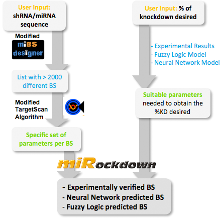 Overview of the miRockdown script flow. The knockdown percentage (kd%) input invokes the selection of the appropriate experimental BS or theoretical binding site parameters. The miRNA sequence starts the generation of BS sequences. Subsequently, these BS sequences are characterized by a modified TargetScan algorithm and finally the parameters of the theoretical BS are compared with the parameters of the generated BSs and the closest of the generated BSs is given as output.
miBSdesignerHaving a binding site designer was crucial to complete the computational approach to our project: miBSdesigner is an easy-to-use application to create in silico binding sites for any given miRNA. Using our device, the user will be able to generate binding sites with several different properties. InputThe user has to input a name for the miRNA to name the primers. The miRNA sequence must be 22 nucleotides long and has to be input in direction 5’ to 3’ (both DNA and RNA sequences are admitted and any extra characters will be removed from the sequence). The user can also enter a spacer inert sequence if he needs to place the binding site further along in the 3’UTR region (it is recommended that the binding site is at least 15 nucleotides away from the stop codon). Initially the user can choose between a perfect binding site (matching the 22 nucleotides), or an almost perfect binding site (matching all of the nucleotides, but leaving a 4-nucleotide bulge between 9 and 12. Apart from these two options, the user can further modify the binding site to meet their individual requirements. Seed Types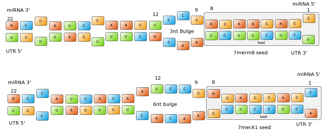 Figure 1: Interactions between two miRNAs and their binding sites with different types of seeds.
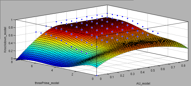
- 6mer (abundance 21.5%): only the nucleotides 2-7 of the miRNA match with the mRNA. - 7merA1 (abundance 15.1%): the nucleotides 2-7 match with the mRNA, and there is an adenine in position 1. - 7merm8 (abundance 25%): the nucleotides 2-8 match with the mRNA. - 8mer (abundance 19.8%): the nucleotides 2-8 match with the mRNA and there is an adenine in position 1. - Apart from any of these options, the user can decide to create a customized seed with one mismatch included. By inputting a number (between 2-7) in the Customized mismatch position textbox The percentages of abundance are calculated among conserved mammalian sites for a highly conserved miRNA [http://2010.igem.org/Team:Heidelberg/Modeling/descriptions#References (Bartel (2009))]. Supplementary RegionIn miBS designer, the user can choose among several types of supplementary regions, starting with 3 matching nucleotides (14-16), increasing sequentially until 8 (13-20), and then total matching (from 13-22, leaving a bulge)[http://2010.igem.org/Team:Heidelberg/Modeling/descriptions#References (Grimson A et al(2007))]. In case the user needs some other specific supplementary region, he can customize the sequence by inputting the desired matching nucleotides (in numbers from 9 to 22, separated by commas). AU ContentIn order to allow the user to improve the efficiency of their binding sites, miBS designer offers options to increase the AU content by adding adenine or uracil to positions around the matches (specifically in -1, 0, 1, 8, 9 and 10). The function is designed so that it varies the AU content without introducing new pairings. Sticky EndsTo facilitate the task of introducing the binding site into a plasmid, the user can add sequences to both ends of the binding site. Initially, the user can choose among the [http://openwetware.org/wiki/The_BioBricks_Foundation:RFC#BBF_RFC_12:_Draft_BioBrick.E2.84.A2_BB-2_standard_for_biological_parts RFC-12 standard for biobricks BB2], the XmaI/XhoI restriction enzymes used in our miTuner-construct, or some custom sequences input by the user. In the last case, the output sequences will not be directly ready for cloning: the user has to either digest the construction prior to ligation, or to process the primers before ordering them to remove the extra nucleotides and create the overhangs. OutputmiBS designer generates the primer needed to integrate the binding site desired into a plasmid, alongside with the primer for the complementary strand. It will also produce specific names for the two primers. mUTINGIt is a tool developed to generate binding sites for miRNAs that could be used for tissue targeting based on both on- as well as off-targeting strategy. It takes as input the target and off-target tissues as well as the desired targeting strategy. User can also specify a threshold for difference in the level of relative expression (within a tissue) of miRNAs between target and off-target tissue. The program searches through a database of expression levels to give out a list of possible miRNAs which could be used. Out of these, the desired miRNA can be selected for which the final output is generated in the form of sense and anti-sense oligomers with overhangs that could be used to put binding sites in tandem or into a vector. InputThe input for the tool is rather simple and consists of five fields. Organism – The tool lets you choose between Human, Rat and Mouse as the source organism. Target – From a list of tissues, the target (tissue where gene has to be expressed) can be selected. Off-target – A list from which multiple off-targets can be selected is available. Here, the tissues from which gene expression has to be excluded can be included. Targeting – This options lets you select the targeting strategy you want to employ. Threshold – The threshold for difference in the level of relative expression of miRNA in the target and off-target tissue can be set here. The default value is 0.001. DataThe expression data and sequence data that the tool makes use of was recruited from preexisting data sources. Sequences – mature miRNA sequences were obtained from mirBase Sequence Database Release 16 [http://2010.igem.org/Team:Heidelberg/Modeling/descriptions#References (Griffiths-Jones S. et al.(2008))]. Expression profiles - miRNA expression profiles were collected from a previously published resource of 172 human, 64 mouse and 16 rat small RNA libraries extracted from major organs and cell types [http://2010.igem.org/Team:Heidelberg/Modeling/descriptions#References (Landgraf et al.(2007))]. The expression values in the data represent the number of cloned mature microRNAs that were sequenced in each library and reported as clone counts. The counts are normalized by the total number of microRNAs that were cloned in each library. These values are then used to calculate the difference in relative miRNA levels for differential expression of the construct. ProcessingThe processing of the data has been done by script written in PERL. After submitting the primary inputs, mentioned above, the tool gives the user a choice of different miRNAs that fulfill the criterion set in the input. These are displayed along with the miRNA expression values in the target (in case of off-targeting) or in the off-targets (in case of on-targeting). The expression values in the off-targets and target in the respective cases are required to be zero. Based on these values, the user can select the most suitable miRNA for their construct. OutputThe final output is the binding site for the miRNA selected by the user. It consists of the sense strand and the anti-sense strand that would code the binding site. These are flanked by a spacer sequence that could be used for putting binding sites in tandem and for introducing cloning sites. ModelingThe Neural Network and the Fuzzy Logic Model explained here are the basis of the miRockdown tool. The results of the optimized models are integrated as a database and enable the miRockdown output of binding sites, to have confidently predicted protein knockdown efficiency. Parameterization ConceptOne of the hardest tasks in the development of our models was to come up with good strategy to generate input parameters from the raw data. In our case, the raw data is the binding site sequence and the corresponding sh/miRNA-sequence. The final parameterization concept unites a basic distinction between perfect, bulged (near-perfect) and endogenous miRNA like BS, with the advanced 3'-scoring and AU-content evaluation. The endogenous miRNA like BS parameter is further split into the three seed-types. The targetscan_scores_50-algorithm [http://2010.igem.org/Team:Heidelberg/Modeling/descriptions#References (Rodriguez et al., 2007)] was used to characterize binding sites in respect to 3'-pairing and AU-content score. TargetScan aligns the miRNA with the mRNA sequence starting from a given seed-position in a way the highest possible 3'-score is reached. Binding from miRNA nucleotide 13-16 will add 1 to the score, pairings outside this region add 0.5. Offsets between bound miRNA and mRNA are also allowed, but will there is a penalty of 0.5 points for an offset higher than 2 nucleotides. The AU-content of 30 nucleotides upstream and downstream of the mRNA seed sequence is rated seed type dependent. The impact of the nucleotides decreases with the distance from the seed. The scoring system is based on a regressions applied to datasets from human, mouse, rat and dog mRNA knockdown [http://2010.igem.org/Team:Heidelberg/Modeling/descriptions#References (Grimson et al., 2007)]. Since all major prior modeling approaches used mRNA levels as training-set, our approach needs to will give a completely new insight into miRNA binding site functionality. These surface fits show the correlation of increasing 3' Binding Score and AU content Score with increasing knockdown-efficiency of the binding sites. Also the other parameters nicely correlate with our expectations.
Neural Network ModelNeural Network theoryArtificial Neural Network usually called (NN), is a computational model that is inspired by the biological nervous system. The network is composed of simple elements called artificial neurons that are interconnected and operate in parallel. In most cases the NN is an adaptive system that can change its structure depending on the internal or and external information that flows into the network during the learning process. The NN can be trained to perform a particular function by adjusting the values of the connection, called weights, between the artificial neurons. Neural Networks have been employed to perform complex functions in various fields, including pattern recognition, identification, classification, speech, vision, and control systems.
Mathematically there are three basic components that describes a single layer network: the synapses of the artificial neurons that are modeled as weights and that represent how strong is the connection between the input and an artificial neuron. An adder, that sum up all the the weighted inputs and finally an activation function, that controls the amplitude of the output of the single layer. Generally there are three type of activation function: threshold, sigmoid, piecewise linear function. For our model the sigmoid function has been used, it can range the output between 0 and 1 or between -1 and 1 [http://2010.igem.org/Team:Heidelberg/Modeling/descriptions#References (Kröse et al, 1996)]. 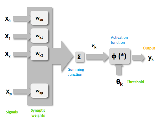 Figure 2: representation of the mathematical model of a biological neuron.
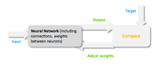 Figure 3: Training of a Neural Network. Model descriptionInput/target pairsThe NN model has been created with the MATLAB NN-toolbox. The input/target pairs used to train the network comprise experimental and literature data [http://2010.igem.org/Team:Heidelberg/Modeling/descriptions#References (Bartel et al., 2007)]. The experimental data were obtained by measuring via luciferase assay the strength of knockdown due to the interaction between the shRNA and the binding site situated on the 3’UTR of luciferase gene (miTuner). Nearly 30 different rational designed binding sites were tested and the respective knockdown strength calculated. Characteristic of the NetworkThe neural network comprised two layers (multilayer feedforward Network). The first layer is connected with the input network and it comprised 15 artificial neurons. The second layer is connected to the first one and it produced the output. For the first and the second layer a sigmoid activation function and a linear activation function were used respectively. The algorithm used for minimizing the cost function (sum squared error) was Resilient Back Propagation (RPROP). RPROP has proven to be one of the best in terms of speed of convergence, moreover it can eliminate the harmful effect of sigmoid activation function used in the hidden layer.
ResultsTwo experiment batches were performed. The network trained only with data coming from literature was used to predict the outcome of the first experiment batch. In Table 1 the simulated and experimental percentage of knockdown are showed. It becomes clear by looking the results that the bulge size has indeed an effect on the knockdown percentage, in fact the network is able to simulate with high precision when the bulge size is on the range of 3 and 4 nt, but not when it becomes 1 or 0. It is important to underly here that the network was trained with literature values that did not take into consideration the bulge size as a key factor, TargetScan in fact, does not evaluate this binding site feature in the scoring process. The importance of the bulge size is also emphasized in the surface plot in the "Parametrization concept" .
Brief conclusionThe bulge size was identified as a very important parameter for knockdown efficiency. This led us to the conclusion of training another Neural Network only with our experimental data and encompassing the bulge size in the input vector.
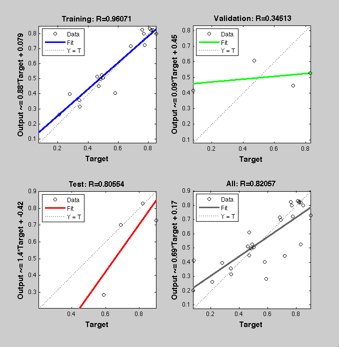
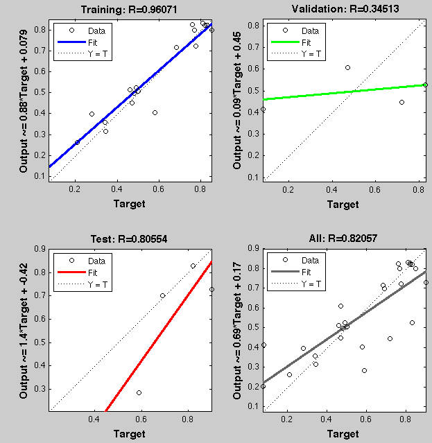
Simulation and experimental verification
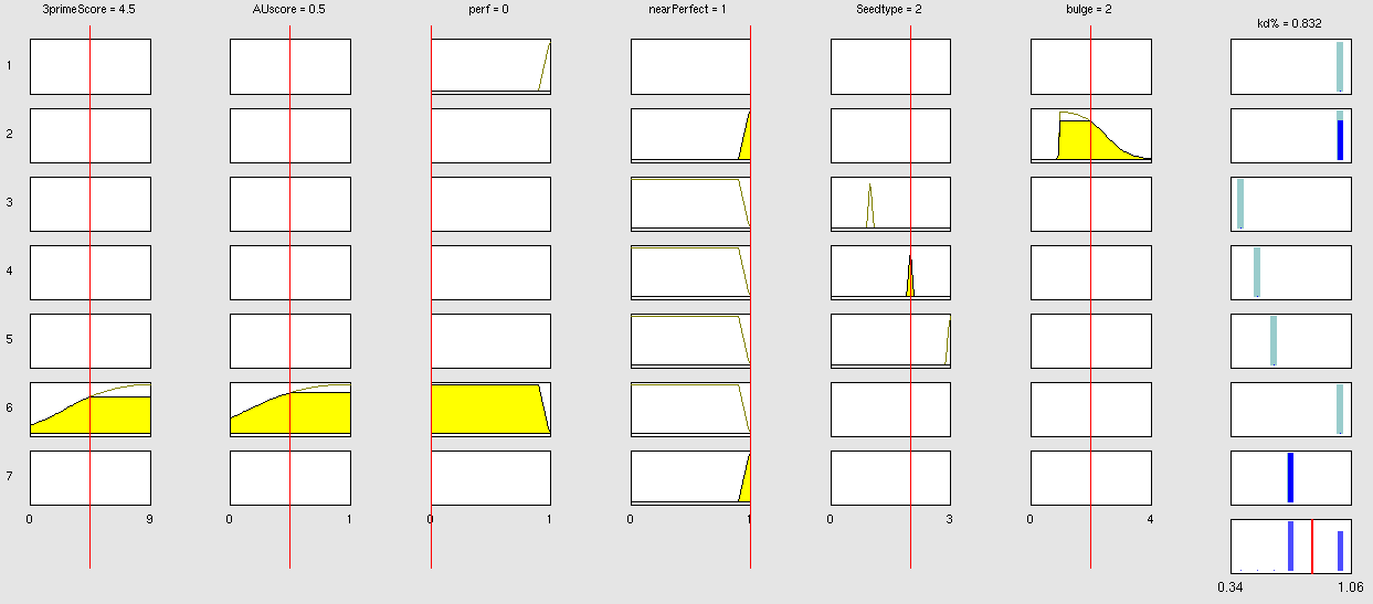
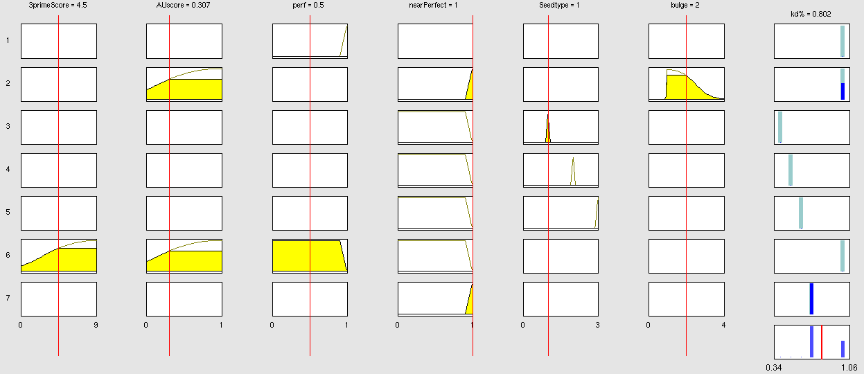
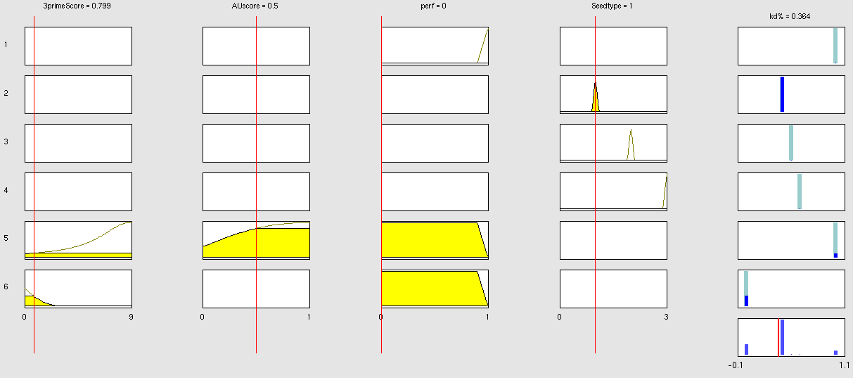
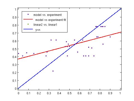
Fuzzy Logic ModelWhy using a fuzzy inference system to model binding site efficiency?To be able to evaluate the complex features of an shRNA or miRNA binding site and predict a resulting knockdown percentage of the protein we developed a fuzzy inference system (fis). The parameterized properties of the binding sites serve as input and will be processed into the knockdown percentage as the single output. Thus our fuzzy inference system is characterized as a multiple input, single output fuzzy inference system (MISO). Fuzzy Logic is a rule-based approximate artificial reasoning method developed by Lotfi Zadeh in 1965. Its motivation is the observation that humans often think and communicate in a vague way, and yet can make precise decisions [http://2010.igem.org/Team:Heidelberg/Modeling/descriptions#References (Nelles O (2000))]. It has been widely used in engineering and Artificial Intelligence approaches such as Fuzzy Controllers and Fuzzy Expert Systems. Fuzzy Logic has also been used for the modeling of biological pathways [http://2010.igem.org/Team:Heidelberg/Modeling/descriptions#References (Bosl et al (2007))] and to analyze gene regulatory networks [http://2010.igem.org/Team:Heidelberg/Modeling/descriptions#References (Laschov et al(2009))]. Key advantages of Fuzzy logic-based approaches are (i) the ability to construct models based on prior knowledge of the system and experimental data and (ii) encode intermediate states for inputs and outputs, thus improving other logic-approaches that can only deal with ON/OFF states such as Boolean models [http://2010.igem.org/Team:Heidelberg/Modeling/descriptions#References (Aldridge et al (2009))] and (iii) simulations can be derived from both qualitative and quantitative data, both of which can be cast into the form of IF-THEN rules. Thus, FL constitutes a powerful approach for the understanding of heterogeneous datasets. Fuzzy inference systems are based on membership functions (MF). MFs rate input parameters how much they satisfy a criterion on a scale from 0 to 1. There can be one, or multiple MFs per input parameter. Like different criteria applied to an input. The height of persons for example can be evaluated with one MF - how much the person satisfies being tall. On the other hand, there could be 3 MFs, one evaluating the membership to small people, the second to medium sized people and the third one to big people. Changing the shape of the MF gives the opportunity to have either functional dependencies, allowing intermediate states of the membership values, or simple ON/OFF states, where the membership value can be only 0 or 1. Thus different kinds of input parameters can be evaluated with a fuzzy inference system. For the simple height example model the age of the person could be taken as second input and evaluated by a MF that is 0 until the age of 18 and 1 for older persons. Thus the model could differentiate between young and grown-up persons. Simple if-then rules can then be used to combine the input MF to an output MF. The satisfaction of a rule by an object (set of input parameters) is defined by the degree of membership of the object to the different MFs. The higher the satisfaction of the rule, the higher is the membership to the output MF. The output MF can be a function like the input MF. This is the case in Mamdani method fuzzy inference systems [http://2010.igem.org/Team:Heidelberg/Modeling/descriptions#References (Mamdani et al, (1975))]. We are using a Sugeno method fuzzy inference system [http://2010.igem.org/Team:Heidelberg/Modeling/descriptions#References (Sugeno(1985))], where the output MF is either a constant or a linear function depending on input parameters. The advantage of a Sugeno fuzzy inference system is, that it is computationally more efficient and easier to optimize or adapt due to the more simple output MF. Due to the non-intuitive combination of the 3'-pairing- and AU-content score, our fuzzy inference system needs to be optimized computationally. Fuzzy Model ConceptsOur fuzzy inference system can deal with 3 different kinds of shRNA binding sites. Perfect, bulged and endogenous-like binding sites are treated separately, due to the differences in their biological mechanism, as discussed earlier [link to binding site properties]. A perfect binding site is evaluated by a simple ON/OFF input MF evaluating the boolean input of We came up with different concepts of what kind of input parameters to integrate into the fuzzy inference model and how to evaluate them. Therefore we parameterized the properties of a large set of binding sites according to various different BS characteristics. The targetscan_50_context_scores – Algorithm [http://2010.igem.org/Team:Heidelberg/Modeling/descriptions#References (Rodriguez et al., 2007)] which evaluates binding sites in respect to 3'-pairing and AU-content gives out a score that seems appropriate to distinguish especially between endogenous miRNA like binding sites. A more detailed description on the concept of binding site parameterization can be found under Model Training Set.
Fuzzy Model OptimizationThe Fuzzy Logic Toolbox and Global Optimization Toolbox were linked via a script and the output membership functions, as well as the input membership function parameters were optimized. Result
Data OverviewThe data used for training the models can be accessed here. It comprises of miRNA and corresponding binding site sequences along with the describing input parameters for the models. References- Bartel D.P., MicroRNAs: Target Recognition and Regulatory Functions, Cell(136):215-233(2009) - Grimson A, Farh KHF, Johnston WK, Garrett-Engele P, Lim LP, Bartel DP, MicroRNA Targeting Specificity in Mammals: Determinants beyond Seed Pairing, Molecular Cell(27):91-105(2007). - Laschov D, Margaliot M. Mathematical modeling of the lambda switch:a fuzzy logic approach. J Theor Biol. 21:475-89 (2009). - Mamdani, E.H. and S. Assilian, An experiment in linguistic synthesis with a fuzzy logic controller. International Journal of Man-Machine Studies, 7(1):1-13, (1975). - Bosl W. J. Systems biology by the rules: hybrid intelligent systems for pathway modeling and discovery. BMC Systems Biology 1:13 (2007). - Sugeno, M., Industrial applications of fuzzy control, Elsevier Science Pub. Co.,(1985). - Nelles O. Nonlinear System Identification Springer Verlag GmbH & Co., Berlin, (2000). - [http://www.targetscan.org/cgi-bin/targetscan/data_download.cgi?db=vert_50 targetscan_50_context_scores.pl] Rodriguez J, Ge R, Walker K, and Bell G., Whitehead Institute for Biomedical Research. (2007,2008) - Kröse B & van der Smagt P, An introduction to Neural Networks, 8th Ed, (1996). - Aldridge B. B., Saez-Rodriguez J., Muhlich J. L., Sorger P. K., Lauffenburger D. A. Fuzzy logic analysis of kinase pathway crosstalk in TNF/EGF/insulin-induced signaling PLoS Comput Biol.5:e1000340 (2009). - MacKay D.J.C., A Practical Bayesian Framework for Backpropagation Networks, Neural Computation, 4(3):448-472(1992) - Landgraf P., Rusu M., Sheridan R., Sewer A., Iovino N., Aravin A., Pfeffer S., Rice A., Kamphorst A.O., Landthaler M., Lin C., Socci N.D., Hermida L., Fulci V., Chiaretti S., Foa R., Schliwka J., Fuchs U., Novosel A., Muller R.U., Schermer B., Bissels U., Inman J., Phan Q., Chien M., A mammalian microRNA expression atlas based on small RNA library sequencing, Cell. 129:1401-1414 (2007). - Griffiths-Jones S., Saini H.K., van Dongen S., Enright A.J. miRBase: tools for microRNA genomics. Nucleic Acid Research. 36:D154-D158 (2008).
|
|||||||||||||||||||||||||||||||||||||||||||||||||||||||||||||||||||||||||||||||||||||||||||||||||||||||||||||||||||||||||||||||||||||||||||||||||||||||||||||||||||||||||||||||||
 "
"
