Team:Michigan/Modeling
From 2010.igem.org
(→Surface Display) |
m (→Oil Sands) |
||
| (34 intermediate revisions not shown) | |||
| Line 2: | Line 2: | ||
<br> | <br> | ||
| - | Mathematical models are very important in the design of an iGEM project. The Michigan modeling team is composed of [[User:Evolver|Josh]], [[User:Kevijose|Kevin]], [[User:htwong|Candy]], [[User:Jejihong|Jennifer]], and [[User:seongkyu|John]] | + | Mathematical models are very important in the design of an iGEM project. The Michigan modeling team is composed of [[User:Evolver|Josh]], [[User:Kevijose|Kevin]], [[User:htwong|Candy]], [[User:Jejihong|Jennifer]], and [[User:seongkyu|John]]. To construct our models, we have taken advantage of MATLAB's Simbiology toolset. More information and tutorials on Matlab and Simbiology can be found here: [http://www.mathworks.com/academia/student_center/tutorials/launchpad.html?s_cid=0410_webg_igem10_294031 MATLAB Tutorial] |
| - | There are several components to a good mathematical model. These include assumptions, parameters, and equations. | + | There are several components to a good mathematical model. These include assumptions, variables, parameters, and equations. |
| + | *Assumptions help to decide how to describe each part of the system, as well as to identify which parts (if any) to deem negligible. Almost always, these assumptions yield an idealized version of the system, and it is within this framework that the model is truly valid. Outside of this ideal model, the real system deviates. However, if the assumptions are sufficiently comprehensive and reasonably valid, then this ideal model can be a very good approximation to the real system. | ||
| + | |||
| + | *Variables are quantities that are "measured" independently, e.g. in a simulation or experiment. As the name implies, they are not defined to be constants in the system, although occasionally a variable may maintain a [nearly] constant value in a particular simulation or trial of an experiment. The behavior, relationships, and responses of the variables are of utmost interest in the model, as they are what allow conclusions to be drawn. | ||
| + | |||
| + | *Parameters are quantities, in particular defined to be constant, that the model takes to be part of the inherent description of the system. They help to characterize the properties and relations between variables. For example, the relationship between two variables is defined by the functional form and the parameters, used as "coefficients". Often, parameters are used to characterize a relationship that cannot or need not be described in an explicit functional form (e.g. reaction rate constants in a differential rate equation). | ||
| + | |||
| + | *Equations relate variables to each other, and they essentially translate the [idealized] system into the language of mathematics. The form of each equation is dictated by the assumptions and the parameters. For example, a system of ordinary differential equations constitutes the mathematical representation of the model. In this case, one seeks the solution to the system of ODEs to acquire a full understanding of the dynamic behavior of the idealized system. Often, an analytic solution may be impossible to find, so numerical simulations/solutions are extensively used. Alternatively, one can examine other aspects, such as steady-state behavior. | ||
==Pili== | ==Pili== | ||
| Line 13: | Line 20: | ||
<u>Assumptions</u> | <u>Assumptions</u> | ||
<br> | <br> | ||
| - | '''There is no growth or degradation of cells | + | '''There is no growth or degradation of cells or algae.''' |
| - | *I made this assumption to simplify the model. | + | *I made this assumption to simplify the model. Because the cells will presumably be in stationary phase by the time they are used as a bioflocculant, this shouldn't make a big difference. |
| - | '''Floc formation only involves two particles | + | '''Floc formation only involves two particles, and collision efficiency is perfect''' |
| - | ''' | + | *This assumption simplifies the model, by removing the need to adjust the parameters to account for the fact that not all collisions between species will result in a floc. |
| - | *This assumption | + | '''All reactions are mass action''' |
| + | *This is a fairly reasonable assumption to model collisions between E. coli and algae based on previous research, although this is greatly simplified [1,2]. | ||
<u>Parameters</u> | <u>Parameters</u> | ||
<br> | <br> | ||
| - | ''' | + | These parameters were determined through running various assays. These parameters are not exact values yet, but are meant to convey a sense of which factors were faster than others. |
| - | *This is | + | '''Rate of piliation= 10''' |
| + | *From experimental observation, the pili growth factor is greater than the rate of flocculation. | ||
| + | '''Rate of algae flocculation= 2.0''' | ||
| + | *The algae appears to flocculate by themselves, and much faster than with the E. coli. This is possibly due to contamination, because the algae is not grown in sterile condition and there could be different species that flocculate. | ||
| + | '''Other flocculation rates= 1.0''' | ||
| + | *It looks like the E. coli flocculate at the same rate with each other. | ||
'''Initial quantities of E. coli and algae are 1 mol.''' | '''Initial quantities of E. coli and algae are 1 mol.''' | ||
| - | *We | + | *In the assays we ran, we used close to a 1:1 volume ratio of cells:algae. This is obviously not ideal for an industrial setting, but we need to experimentally prove that our idea will work. |
| + | |||
| + | [[Image:Pili_floc_model.jpg|500px]] | ||
| + | |||
| + | ===Conclusions and Further Work=== | ||
| + | This results graph shows that the population of both the algae and the flocs stabilize to a constant level over time. We need to conduct more laboratory assays to determine if this is the actual case. If it is, we can adjust the model and start running more simulations to relate it to the lab setting. Possible solutions to increase the amount of the flocs would be to add more E. coli, but this is not ideal in the industrial setting due to the cost. | ||
| + | [[#top|Back to top]] | ||
<br style="clear: both" /> | <br style="clear: both" /> | ||
==Quorum Sensing== | ==Quorum Sensing== | ||
| - | Quorum sensing has been modeled by other iGEM teams for previous competitions, including: [ | + | Quorum sensing has been modeled by other iGEM teams for previous competitions, including: [https://2007.igem.org/Bangalore Bangalore] and [https://2008.igem.org/Team:NTU-Singapore Singapore] |
[[Image:LuxS- Modeling001.jpg|right]] This model is based on the paper [http://jb.asm.org/cgi/content/short/189/16/6011 Quorum Sensing in Escherichia coli Is Signaled by AI-2/LsrR: Effects on Small RNA and Biofilm Architecture (doi:10.1128/JB.00014-07)] and was created with the help of [[User:infekt|Alex]] who is also on the quorum sensing team. More information about quorum sensing can be found here: [[Team:Michigan/Project]] and their notebook can be found here: [[Team:Michigan/Quorum_Sensing]]. | [[Image:LuxS- Modeling001.jpg|right]] This model is based on the paper [http://jb.asm.org/cgi/content/short/189/16/6011 Quorum Sensing in Escherichia coli Is Signaled by AI-2/LsrR: Effects on Small RNA and Biofilm Architecture (doi:10.1128/JB.00014-07)] and was created with the help of [[User:infekt|Alex]] who is also on the quorum sensing team. More information about quorum sensing can be found here: [[Team:Michigan/Project]] and their notebook can be found here: [[Team:Michigan/Quorum_Sensing]]. | ||
| Line 66: | Line 85: | ||
<br> | <br> | ||
<br> | <br> | ||
| - | + | [[#top|Back to top]] | |
<br style="clear: both" /> | <br style="clear: both" /> | ||
==Surface Display== | ==Surface Display== | ||
| - | [[Image:diagram.jpg|400px]] | + | [[Image:diagram.jpg|400px|left|thumb|fig.1 the diagram of the model]] |
<br style="clear: both" /> | <br style="clear: both" /> | ||
This model predicts the behavior of an algae specific binding protein expressed by E. Coli. It is relevant to vp130 project described [https://2010.igem.org/Team:Michigan/Project#Hy-Bi:_Virus_Protein_Surface_Display here]. | This model predicts the behavior of an algae specific binding protein expressed by E. Coli. It is relevant to vp130 project described [https://2010.igem.org/Team:Michigan/Project#Hy-Bi:_Virus_Protein_Surface_Display here]. | ||
| Line 96: | Line 115: | ||
| + | [[Image:flocculation.jpg|right|550px|thumb|fig.2 a simulation with the rate constants mentioned above]] | ||
<b>Parameters</b> | <b>Parameters</b> | ||
| Line 101: | Line 121: | ||
1. Significant rate constants | 1. Significant rate constants | ||
| - | * Forward flocculation: | + | * Forward flocculation: 100.0 / (mol x sec) |
* Reverse flocculation: 1.0 / (sec) | * Reverse flocculation: 1.0 / (sec) | ||
* Surface protein expression: 100.0 / (mol x sec) | * Surface protein expression: 100.0 / (mol x sec) | ||
| Line 111: | Line 131: | ||
* Algae: 1 mol | * Algae: 1 mol | ||
| - | |||
| - | + | <b>Application</b> | |
| + | Currently, the graph for flocculation looks sigmoidal, but it can be made exponential by growing algae and E.Coli on separate media. | ||
| + | [[#top|Back to top]] | ||
<br style="clear: both" /> | <br style="clear: both" /> | ||
| Line 194: | Line 215: | ||
Note: Although concentration and time are in arbitrary units, they are consistent across all plots. | Note: Although concentration and time are in arbitrary units, they are consistent across all plots. | ||
| - | [[Image: | + | [[Image:log_dec_NAs.jpg|500px]] |
| - | + | ||
| - | + | ||
[[Image:influent entry unlim nutr.jpg|500px]] | [[Image:influent entry unlim nutr.jpg|500px]] | ||
| Line 202: | Line 221: | ||
[[Image:decline of pseudo pop in res.jpg|550px]] | [[Image:decline of pseudo pop in res.jpg|550px]] | ||
| + | |||
| + | '''Conclusions''' | ||
| + | |||
| + | From this model, we can extrapolate that the longer the bioreactor, the more NAs will be degraded, as the ''Pseudomonas'' species are present along the entire length of the bioreactor. We also find that, when described with a logistic equation, ''Pseudomonas'' populations eventually reached a steady state in each unit, coupled with the plateau of NA concentration in the corresponding units. In future studies, if an estimate of NA degradation efficiency is described along the length of the bioreactor, we can model NA degradation assuming that ''Pseudomonas'' population are in a steady state. In addition, it is made clear in the semi-log plot of NA concentration of each unit that efficiency per length of bioreactor in degrading NAs decrease exponentially. It is thus unnecessary to produce a bioreactor beyond a certain length, where the NAs degraded along the additional length contribute very little to the NA concentration in the effluent. | ||
Ideally, a drip flow bioreactor should be modeled by a plug flow reactor model, which describes a fluid flowing through a pipe with perfect mixing in the radial direction and no mixing in the axial direction. However, we deemed the method above to be sufficient for our purposes and more intuitive in design. [https://2009.igem.org/Team:uOttawa/Modeling uOttawa] used plug flow model to describe nutrient flow in the intestines. | Ideally, a drip flow bioreactor should be modeled by a plug flow reactor model, which describes a fluid flowing through a pipe with perfect mixing in the radial direction and no mixing in the axial direction. However, we deemed the method above to be sufficient for our purposes and more intuitive in design. [https://2009.igem.org/Team:uOttawa/Modeling uOttawa] used plug flow model to describe nutrient flow in the intestines. | ||
| + | |||
| + | [[#top|Back to top]] | ||
==References== | ==References== | ||
1. Kuwahara, H., Myers, C., Samoilov, M., Abstracted Stochastic Analysis of Type 1 Pili Expression in E. Coli. | 1. Kuwahara, H., Myers, C., Samoilov, M., Abstracted Stochastic Analysis of Type 1 Pili Expression in E. Coli. | ||
| - | 2. | + | 2. Wolf, D., and Arkin, A., Fifteen Minutes of ''fim'': Control of Type 1 Pili Expression in E. Coli. OMICS 6 2002 |
| - | 3. | + | 3. [http://jb.asm.org/cgi/content/short/189/16/6011 Li, J., C. Attila, L. Wang, T. K. Wood, J. J. Valdes, and W. E. Bentley. 2007. Quorum sensing in Escherichia coli is signaled by AI-2/LsrR: effects on small RNA and biofilm architecture. J. Bacteriol. 189:6011-6020.] |
4. [http://www.ncbi.nlm.nih.gov/pubmed/17040229 Del Rio, L., Hadwin, A., Pinto, L., MacKinnon, M. and Moore, M. (2006), Degradation of naphthenic acids by sediment micro-organisms. Journal of Applied Microbiology, 101: 1049–1061.] | 4. [http://www.ncbi.nlm.nih.gov/pubmed/17040229 Del Rio, L., Hadwin, A., Pinto, L., MacKinnon, M. and Moore, M. (2006), Degradation of naphthenic acids by sediment micro-organisms. Journal of Applied Microbiology, 101: 1049–1061.] | ||
Latest revision as of 05:30, 27 October 2010
Mathematical models are very important in the design of an iGEM project. The Michigan modeling team is composed of Josh, Kevin, Candy, Jennifer, and John. To construct our models, we have taken advantage of MATLAB's Simbiology toolset. More information and tutorials on Matlab and Simbiology can be found here: [http://www.mathworks.com/academia/student_center/tutorials/launchpad.html?s_cid=0410_webg_igem10_294031 MATLAB Tutorial]
There are several components to a good mathematical model. These include assumptions, variables, parameters, and equations.
- Assumptions help to decide how to describe each part of the system, as well as to identify which parts (if any) to deem negligible. Almost always, these assumptions yield an idealized version of the system, and it is within this framework that the model is truly valid. Outside of this ideal model, the real system deviates. However, if the assumptions are sufficiently comprehensive and reasonably valid, then this ideal model can be a very good approximation to the real system.
- Variables are quantities that are "measured" independently, e.g. in a simulation or experiment. As the name implies, they are not defined to be constants in the system, although occasionally a variable may maintain a [nearly] constant value in a particular simulation or trial of an experiment. The behavior, relationships, and responses of the variables are of utmost interest in the model, as they are what allow conclusions to be drawn.
- Parameters are quantities, in particular defined to be constant, that the model takes to be part of the inherent description of the system. They help to characterize the properties and relations between variables. For example, the relationship between two variables is defined by the functional form and the parameters, used as "coefficients". Often, parameters are used to characterize a relationship that cannot or need not be described in an explicit functional form (e.g. reaction rate constants in a differential rate equation).
- Equations relate variables to each other, and they essentially translate the [idealized] system into the language of mathematics. The form of each equation is dictated by the assumptions and the parameters. For example, a system of ordinary differential equations constitutes the mathematical representation of the model. In this case, one seeks the solution to the system of ODEs to acquire a full understanding of the dynamic behavior of the idealized system. Often, an analytic solution may be impossible to find, so numerical simulations/solutions are extensively used. Alternatively, one can examine other aspects, such as steady-state behavior.
Pili
We have decided to model the growth of a biofilm using pili. By modeling the flocculation of the algae, we hope to be able to predict how our reactions will proceed and determine quantities such as the optimal initial concentration of E. coli.
Assumptions
There is no growth or degradation of cells or algae.
- I made this assumption to simplify the model. Because the cells will presumably be in stationary phase by the time they are used as a bioflocculant, this shouldn't make a big difference.
Floc formation only involves two particles, and collision efficiency is perfect
- This assumption simplifies the model, by removing the need to adjust the parameters to account for the fact that not all collisions between species will result in a floc.
All reactions are mass action
- This is a fairly reasonable assumption to model collisions between E. coli and algae based on previous research, although this is greatly simplified [1,2].
Parameters
These parameters were determined through running various assays. These parameters are not exact values yet, but are meant to convey a sense of which factors were faster than others.
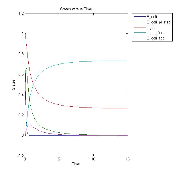
Rate of piliation= 10
- From experimental observation, the pili growth factor is greater than the rate of flocculation.
Rate of algae flocculation= 2.0
- The algae appears to flocculate by themselves, and much faster than with the E. coli. This is possibly due to contamination, because the algae is not grown in sterile condition and there could be different species that flocculate.
Other flocculation rates= 1.0
- It looks like the E. coli flocculate at the same rate with each other.
Initial quantities of E. coli and algae are 1 mol.
- In the assays we ran, we used close to a 1:1 volume ratio of cells:algae. This is obviously not ideal for an industrial setting, but we need to experimentally prove that our idea will work.
Conclusions and Further Work
This results graph shows that the population of both the algae and the flocs stabilize to a constant level over time. We need to conduct more laboratory assays to determine if this is the actual case. If it is, we can adjust the model and start running more simulations to relate it to the lab setting. Possible solutions to increase the amount of the flocs would be to add more E. coli, but this is not ideal in the industrial setting due to the cost.
Quorum Sensing
Quorum sensing has been modeled by other iGEM teams for previous competitions, including: Bangalore and Singapore
This model is based on the paper [http://jb.asm.org/cgi/content/short/189/16/6011 Quorum Sensing in Escherichia coli Is Signaled by AI-2/LsrR: Effects on Small RNA and Biofilm Architecture (doi:10.1128/JB.00014-07)] and was created with the help of Alex who is also on the quorum sensing team. More information about quorum sensing can be found here: Team:Michigan/Project and their notebook can be found here: Team:Michigan/Quorum_Sensing.This model shows the movement of AI2 (Autoinducer-2) from outside the cell (AI2_o) to inside the cell (AI2_i). The final output after transcription and translation is GFP in the case of the Lux- mutants recieved; however, at the end of the project, this will hopefully cause flocculation of the microalgae.
This model is also specific to the Lux- mutants as it is not understood how LuxS works or is produced. [http://jb.asm.org/cgi/content/short/189/16/6011 (doi:10.1128/JB.00014-07)]
Assumptions
- Assume all massaction
- This greatly simplifies the model and gives a good estimate; however, it is unrealistic.
- Initially, all LsrR bound to all operators to inhibit.
- This also simplifies the model.
- Creation of LsrS is unknown so simply exists in the cell at a fixed concentration. Any output that occurs is due to the addition of AI2 from the person performing the experiment.
- Assume that the proteins that bring in AI2 (Lsr A, B, C, and D) exist in a protein complex and can be called one "species" in Matlab. Also assume that the protein complex is created and formed at the same time.
- This simplifies the number of species in Matlab and also simplifies the model.
- Assuming no degradation for now... Molecule is "used" up in reaction.
- This simplifies the model by removing degradation from the equations.
Parameters
- For now, all rate constants are 1.
- This simplifies the model; however, it is not realistic.
- Assumptions with quantities
- A lot of AI2_o in comparison with all other molecules.
- This is saying that the experimenter will add a higher concentration of AI2 than the concentrations of various molecules that exist in the cell.
- Initially low concentration of Lsr A,B,C,D transport proteins
- Low basal expression of the transport proteins.
- Low concentration of LsrK
- Low basal expression of LsrK.
- Low concentration of LsrR + Operator
- In comparison with the protein concentration, the number of plasmids containing the Operator is low.
- A lot of AI2_o in comparison with all other molecules.
Since the Quorum Sensing Team is only measuring the output of GFP from the addition of AI2, this is the output that really matters. As can be seen, after a certain amount of time, the expression of GFP levels off.
Back to top
Surface Display
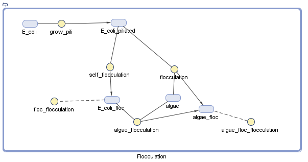
This model predicts the behavior of an algae specific binding protein expressed by E. Coli. It is relevant to vp130 project described here.
Assumptions
1-1. The flocculation depends on only the concentrations of algae and flocculant.
1-2. The flocculation depends on only the collision between species with surface proteins and algae
2. The forward reaction for flocculation is much faster than the reverse reaction.
3-1. Flocculated species are invincible--they do not die.
3-2. Other species, such as unexpressed/expressed species and algae, also do not die.
- Our model takes into account the deaths for all the species mention above, but the constants were made not functional during the simulation.
4. Algae and unexpressed/expressed species are assumed to grow on the same media.
- However, if necessary, our model can assume that they grow on separate media and then added together to flocculate.
5. The expression of surface proteins is based on solely the amount of "unexpressed" species and the concentration of media.
Parameters
1. Significant rate constants
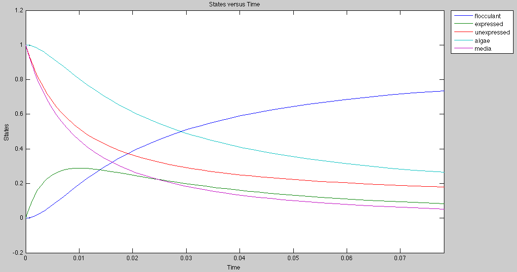
- Forward flocculation: 100.0 / (mol x sec)
- Reverse flocculation: 1.0 / (sec)
- Surface protein expression: 100.0 / (mol x sec)
2. Initial concentrations
- Media: 1 mol
- Unexpressed species: 1 mol
- Algae: 1 mol
Application
Currently, the graph for flocculation looks sigmoidal, but it can be made exponential by growing algae and E.Coli on separate media.
Back to top
Oil Sands
We are developing a mathematical model which describes the degradation of naphthenic acids (NAs) by Pseudomonas putida and Pseudomonas fluorescens in a biofilm in a drip flow bioreactor under aerobic conditions. We will use a series of [http://controls.engin.umich.edu/wiki/index.php/Bacterial_Chemostat_Model chemostat] models to approximate the change in NA concentration along the length of the bioreactor and through time.
In developing the mathematical model, we made the following assumptions:
- Our models will assume a homogeneous mixture of P. putida and P. fluorescens and represent the two species as one organism.
- It is known that P. putida and P. fluorescens synergistically degrade NAs [4]. The mechanism of the synergistic degradation and differentiation between the two species should have little effect in evaluating the efficiency of NA degradation.
- The biofilm is always distributed homogeneously throughout the bioreactor, and diffusion of NAs into the biofilm occurs instantaneously.
- This assumption is made to simplify the model.
- We assume that NAs remain in solution within the bioreactor.
- NAs are not known to be volatile.
- The density ratio of the two Pseudomonas species do not fluctuate.
- This assumption is likely unrealistic.
- Oxygen is not a limiting substrate.
- Area of cross sections remain unchanged through the length of bioreactor.
Reactions
The system is represented by nine repeating units of the following reactions, with the units distinguished by a number n: 0 =< n =< 8. All reactions are assumed to be mass action. For n = 0, there is no NA_n-1 -> NA_n and NA_n is a constant.
The flow of NA from one unit to the next is described simply with a mass action model:
dNA_n = kinflow_n-1*NA_n-1 - kinflow_n*NA_n
As the velocity of the liquid is constant throughout the model, kinflow_n-1 = kinflow_n.
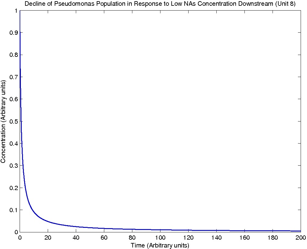
Pseudomonas population is modeled by the logistic growth curve, yielding
dPseudo_n/dt = kdegrade*NA_n*Pseudo_n - kdeath*(Pseudo_n)^2
| Rate: | Value: |
| kinflow | 0.1 |
| kdegrade | 10.0 |
| kdeath | 1.0 |
| Initial value: | Note: | Value: |
| NA_0 | A constant | 0.5 |
| NA_n | n > 0 | 0.0 |
| Pseudo_n | 1.0 |
Results
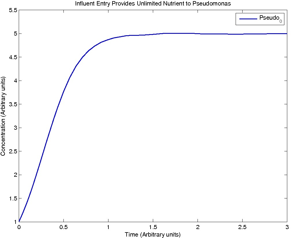
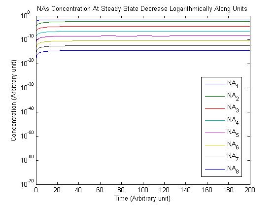
Note: Although concentration and time are in arbitrary units, they are consistent across all plots.
Conclusions
From this model, we can extrapolate that the longer the bioreactor, the more NAs will be degraded, as the Pseudomonas species are present along the entire length of the bioreactor. We also find that, when described with a logistic equation, Pseudomonas populations eventually reached a steady state in each unit, coupled with the plateau of NA concentration in the corresponding units. In future studies, if an estimate of NA degradation efficiency is described along the length of the bioreactor, we can model NA degradation assuming that Pseudomonas population are in a steady state. In addition, it is made clear in the semi-log plot of NA concentration of each unit that efficiency per length of bioreactor in degrading NAs decrease exponentially. It is thus unnecessary to produce a bioreactor beyond a certain length, where the NAs degraded along the additional length contribute very little to the NA concentration in the effluent.
Ideally, a drip flow bioreactor should be modeled by a plug flow reactor model, which describes a fluid flowing through a pipe with perfect mixing in the radial direction and no mixing in the axial direction. However, we deemed the method above to be sufficient for our purposes and more intuitive in design. uOttawa used plug flow model to describe nutrient flow in the intestines.
References
1. Kuwahara, H., Myers, C., Samoilov, M., Abstracted Stochastic Analysis of Type 1 Pili Expression in E. Coli.
2. Wolf, D., and Arkin, A., Fifteen Minutes of fim: Control of Type 1 Pili Expression in E. Coli. OMICS 6 2002
3. [http://jb.asm.org/cgi/content/short/189/16/6011 Li, J., C. Attila, L. Wang, T. K. Wood, J. J. Valdes, and W. E. Bentley. 2007. Quorum sensing in Escherichia coli is signaled by AI-2/LsrR: effects on small RNA and biofilm architecture. J. Bacteriol. 189:6011-6020.]
4. [http://www.ncbi.nlm.nih.gov/pubmed/17040229 Del Rio, L., Hadwin, A., Pinto, L., MacKinnon, M. and Moore, M. (2006), Degradation of naphthenic acids by sediment micro-organisms. Journal of Applied Microbiology, 101: 1049–1061.]
 "
"

