 "
"
Team:Aberdeen Scotland/Curve Fitting
From 2010.igem.org
(Difference between revisions)
| Line 15: | Line 15: | ||
</right> | </right> | ||
<left> | <left> | ||
| - | <p style="font-size:10px">Figure 5. A. Graph from paper by Witherell et al.[14] showing the binding curves of the MS2 stem loop. The filled squares are the 8-16 construct<br> which closely resembles the binding curves of our MS2 stems. B. The binding curve for the 8-16 construct was reproduced in MATLAB and the Hill function for activators equation fitted to it (red line). </p> | + | <p style="font-size:10px">Figure 5. A. Graph from paper by Witherell et al.[14] showing the binding curves of the MS2 stem loop. The filled squares are the 8-16 construct<br> which closely resembles the binding curves of our MS2 stems. B. The binding curve for the 8-16 construct was reproduced in MATLAB and the Hill<br> function for activators equation fitted to it (red line). </p> |
</left> | </left> | ||
</html> | </html> | ||
Revision as of 13:57, 20 October 2010
University of Aberdeen - ayeSwitch
iGEM 2010
Curve Fitting to find the Hill Coefficient for the GFP/Bbox-stem Association (n2)
Based on a graph in a paper by Witherell et al.[14] which showed the binding curves of the MS2 stem loop we could calculate more accurately the value for n1. Our two MS2 stem loops (see Fig 1 in Equations) are 19 nucleotides apart, so our binding curve will most closely resemble that of the 8-16 construct, shown in figure 5A (filled squares).
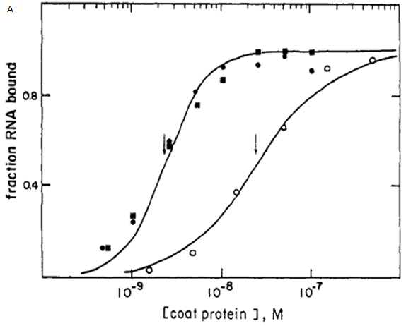
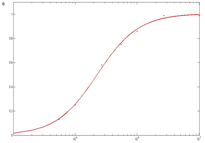
Figure 5. A. Graph from paper by Witherell et al.[14] showing the binding curves of the MS2 stem loop. The filled squares are the 8-16 construct
which closely resembles the binding curves of our MS2 stems. B. The binding curve for the 8-16 construct was reproduced in MATLAB and the Hill
function for activators equation fitted to it (red line).